
Find the general solution to \(x^{2}y^{\prime \prime }+3xy^{\prime }+y=\frac{4}{x}\)
Solution: This is Euler differential equation. The homogeneous solution \(y_{h}\) is first found, then variation of parameters method is used to find the particular solution \(y_{p}\). The general solution can then be written as \(y=y_{h}+y_{p}\)
Comparing the homogeneous part to the standard form of Euler differential equation, which is given by\[ x^{2}y^{\prime \prime }+Axy^{\prime }+By=0 \] Where in the above \(y(x)\) is a function of \(x,\) shows that \(A=3\) and \(B=1\).
Applying the transformation1 \(t=\ln (x)\) to the original ODE converts it to\begin{align} y^{\prime \prime }+(A-1)y^{\prime }+By & =0\nonumber \\ y^{\prime \prime }+2y^{\prime }+y & =0 \tag{1} \end{align}
Where \(y(t)\) is now a function of \(t\) and not \(x\). This new ODE is solved for \(y(t)\). The solution is then converted back to be a function of \(x\).
Since Eq. (1) now is a constant coefficients ODE, direct application of characteristic roots method can be used. The roots of \(\lambda ^{2}+2\lambda +1=0\) are \(\lambda =\frac{-b\pm \sqrt{b^{2}-4ac}}{2a}=\frac{-2\pm \sqrt{4-4}}{2}=-1\) (repeated). Therefore the solution to Eq. (1) is\[ y(t)=c_{1}e^{-t}+c_{2}te^{-t}\] The above solution is converted back to be a function of \(x\) using \(t=\ln (x).\)This results in \begin{align} y_{h}\left ( x\right ) & =c_{1}e^{-\ln \left ( x\right ) }+c_{2}\ln \left ( x\right ) e^{-\ln \left ( x\right ) }\nonumber \\ & =\frac{c_{1}}{x}+c_{2}\frac{\ln \left ( x\right ) }{x} \tag{2} \end{align}
This is valid for \(x>0\) and \(x<0\) but not for \(x=0\). The solution can also be written as\[ y_{h}\left ( x\right ) =\frac{c_{1}}{x}+c_{2}\frac{\ln \left ( \left \vert x\right \vert \right ) }{x}\] Now that the homogeneous solution is found, the particular solution is obtained using variation of parameters. Let the two linearly independent solutions of the homogeneous part of the solution to the ODE as shown in Eq. (2) be \begin{align*} y_{1} & =\frac{1}{x}\\ y_{2} & =\frac{\ln \left ( x\right ) }{x} \end{align*}
The particular solution \(y_{p}\) is\[ y_{p}=u_{1}y_{1}+u_{2}y_{2}\] Where \(u_{1},u_{2}\) are two functions to be determined. Using the standard formula derived in class, these functions are \begin{align} u_{1} & =\int \frac{-y_{2}}{W\left ( x\right ) }\frac{f\left ( x\right ) }{a_{0}}dx\tag{1}\\ u_{2} & =\int \frac{y_{1}}{W\left ( x\right ) }\frac{f\left ( x\right ) }{a_{0}}dx \tag{2} \end{align}
Where \(f\left ( x\right ) =\frac{4}{x}\) and \(a_{0}=x^{2}\). The Wronskian is\begin{align*} W\left ( x\right ) & =\begin{vmatrix} y_{1} & y_{2}\\ y_{1}^{\prime } & y_{2}^{\prime }\end{vmatrix} =\begin{vmatrix} \frac{1}{x} & \frac{\ln \left ( x\right ) }{x}\\ -\frac{1}{x^{2}} & -\frac{1}{x^{2}}\ln \left ( x\right ) +\frac{1}{x^{2}}\end{vmatrix} =\frac{1}{x}\left ( -\frac{1}{x^{2}}\ln \left ( x\right ) +\frac{1}{x^{2}}\right ) +\left ( \frac{1}{x^{2}}\right ) \frac{\ln \left ( x\right ) }{x}\\ & =-\frac{\ln \left ( x\right ) }{x^{3}}+\frac{1}{x^{3}}+\frac{\ln \left ( x\right ) }{x^{3}}\\ & =\frac{1}{x^{3}} \end{align*}
\(u_{1}\) is found from Eq (1)\begin{align*} u_{1} & =\int \frac{-\frac{\ln \left ( x\right ) }{x}}{\frac{1}{x^{3}}}\frac{\frac{4}{x}}{x^{2}}dx=-4\int \frac{\ln \left ( x\right ) }{x}dx=-4\left ( \frac{\ln \left ( x\right ) ^{2}}{2}\right ) \\ & =-2\ln \left ( x\right ) ^{2} \end{align*}
\(u_{2}\) is found from Eq. (2)\begin{align*} u_{2} & =\int \frac{\frac{1}{x}}{\frac{1}{x^{3}}}\frac{\frac{4}{x}}{x^{2}}dx=4\int \frac{1}{x}dx\\ & =4\ln \left ( x\right ) \end{align*}
Therefore the particular solution becomes\begin{align*} y_{p} & =u_{1}y_{1}+u_{2}y_{2}\\ & =-2\ln \left ( x\right ) ^{2}\frac{1}{x}+4\ln \left ( x\right ) \frac{\ln \left ( x\right ) }{x}\\ & =-2\frac{\ln \left ( x\right ) ^{2}}{x}+4\frac{\ln \left ( x\right ) ^{2}}{x}\\ & =2\frac{\ln \left ( x\right ) ^{2}}{x} \end{align*}
And finally the general solution is obtained\begin{align*} y & =y_{h}+y_{p}\\ & =\frac{c_{1}}{x}+c_{2}\frac{\ln \left ( x\right ) }{x}+2\frac{\ln \left ( x\right ) ^{2}}{x} \end{align*}
Hence \[ y=\frac{1}{x}\left ( c_{1}+c_{2}\ln \left ( x\right ) +2\ln \left ( x\right ) ^{2}\right ) \]
Using variation of parameters, show that \[ y=c_{1}\cosh (kx)+c_{2}\sinh (kx)+\frac{1}{k}\int _{0}^{x}\sinh (k(x-s))\,f(s)\,ds \] Is a complete solution of the equation \(y^{\prime \prime }-k^{2}y=f(x)\), where \(k\neq 0\) and \(f\) is everywhere continuous. Hint: Introduce the dummy variable \(s\) in the integrals which define \(u_{1}\) and \(u_{2}\). Then move \(y_{1}(x)\) and \(y_{2}(x)\) into the integrands of the respective integrals and combine the two integrals.
solution: Since the ODE is constant coefficients, direct application of the roots of the characteristic equation is used to obtain the homogeneous solution \(y_{h}\). The roots of the characteristic equation are \(\lambda =\frac{-b\pm \sqrt{b^{2}-4ac}}{2a}=\frac{\pm \sqrt{4k^{2}}}{2}=\pm k\), hence\begin{align*} y_{h} & =c_{1}e^{kx}+c_{2}e^{-kx}\\ & =c_{1}\cosh \left ( kx\right ) +c_{2}\sin \left ( kx\right ) \end{align*}
Let \begin{align*} y_{1} & =\cosh \left ( kx\right ) \\ y_{2} & =\sinh \left ( kx\right ) \end{align*}
The Wronskian is \begin{align*} W\left ( x\right ) & =\begin{vmatrix} y_{1} & y_{2}\\ y_{1}^{\prime } & y_{2}^{\prime }\end{vmatrix} =\begin{vmatrix} \cosh \left ( kx\right ) & \sinh \left ( kx\right ) \\ k\sinh \left ( kx\right ) & k\cosh \left ( kx\right ) \end{vmatrix} =k\cosh \left ( x\right ) ^{2}+k\sinh \left ( kx\right ) ^{2}\\ & =k \end{align*}
Let the particular solution be\[ y_{p}=u_{1}y_{1}+u_{2}y_{2}\] hence\begin{align} u_{1} & =\int \frac{-y_{2}}{W\left ( x\right ) }\frac{f\left ( x\right ) }{a_{0}}dx\tag{1}\\ u_{2} & =\int \frac{y_{1}}{W\left ( x\right ) }\frac{f\left ( x\right ) }{a_{0}}dx \tag{2} \end{align}
Therefore\begin{align*} u_{1} & =\int \frac{-\sinh \left ( kx\right ) }{k}f\left ( x\right ) dx\\ u_{2} & =\int \frac{\cosh \left ( kx\right ) }{k}f\left ( x\right ) dx \end{align*}
Applying Eqs. (1) and (2) gives the particular solution \[ y_{p}=\frac{1}{k}\cosh \left ( kx\right ) \left ( \int -\sinh \left ( kx\right ) f\left ( x\right ) dx\right ) +\frac{1}{k}\sinh \left ( kx\right ) \left ( \int \cosh \left ( kx\right ) f\left ( x\right ) dx\right ) \] Let \(s=x\), hence \(ds=dx\). The integration remains non-definite and can now be written as\[ y_{p}=\frac{1}{k}\cosh \left ( kx\right ) \left ( \int -\sinh \left ( ks\right ) f\left ( s\right ) ds\right ) +\frac{1}{k}\sinh \left ( kx\right ) \left ( \int \cosh \left ( ks\right ) f\left ( s\right ) ds\right ) \] Now \(\cosh \left ( kx\right ) \) and \(\sinh \left ( kx\right ) \) can be moved inside the integrals since they do not depend on the new dummy variable \(s\) and are hence treated as constants inside the integration. This results in\begin{align} y_{p} & =\frac{1}{k}\left ( \int -\cosh \left ( kx\right ) \sinh \left ( ks\right ) f\left ( s\right ) ds\right ) +\frac{1}{k}\left ( \int \sinh \left ( kx\right ) \cosh \left ( ks\right ) f\left ( s\right ) ds\right ) \nonumber \\ & =\frac{1}{k}\int \left ( \sinh \left ( kx\right ) \cosh \left ( ks\right ) -\cosh \left ( kx\right ) \sinh \left ( ks\right ) \right ) \ f\left ( s\right ) \ ds \tag{3} \end{align}
Using the trigonometric relation\[ \sinh A\cosh B-\cosh A\sinh B=\sinh \left ( A-B\right ) \] Eq. (3) becomes\[ y_{p}=\frac{1}{k}\int \sinh \left ( k\left ( x-s\right ) \right ) \ f\left ( s\right ) \ ds \] Therefore, the general solution is\begin{align*} y & =y_{h}+y_{p}\\ & =c_{1}\cosh \left ( kx\right ) +c_{2}\sin \left ( kx\right ) +\frac{1}{k}\int \sinh \left ( k\left ( x-s\right ) \right ) \ f\left ( s\right ) \ ds \end{align*}
which is what was asked to show. Note: The question asks to show the final integral as definite with limits \(\int _{0}^{x}.\) However in the solution obtained above, the integral is non-definite \(\int \). Need more clarification on this point.
Problem 8, page 72: Verify that the given function is a solution of the differential equation. Derive the equation
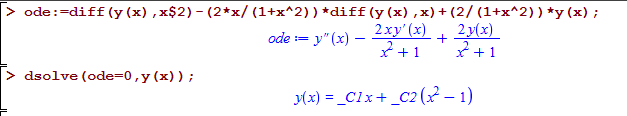
satisfied by \(u(x)\), give its solution and give the general solution of the second order equation: \(y^{\prime \prime }-\frac{2x}{1+x^{2}}y^{\prime }+\frac{2}{1+x^{2}}y=0;y_{1}\left ( x\right ) =x\)
Solution:
Let the second solution of the ODE be \(y_{2}=uy_{1}\) where \(u\left ( x\right ) \) is a function of \(x\) to be determined. The derivatives of \(y_{2}\) are now found and substituted back into the ODE to solve for \(u\).\begin{align} y_{2}^{\prime } & =u^{\prime }y_{1}+uy_{1}^{\prime }\tag{1}\\ y_{2}^{\prime \prime } & =u^{\prime \prime }y_{1}+u^{\prime }y_{1}^{\prime }+u^{\prime }y_{1}^{\prime }+uy_{1}^{\prime \prime } \tag{2} \end{align}
Since \(y_{2}\) is assumed to be a solution of the original ODE, then it satisfies it. Hence\begin{equation} y_{2}^{\prime \prime }-\frac{2x}{1+x^{2}}y_{2}^{\prime }+\frac{2}{1+x^{2}}y_{2}=0 \tag{3} \end{equation} Using Eqs. (1) and (2) into (3) gives\begin{align*} \left ( u^{\prime \prime }y_{1}+u^{\prime }y_{1}^{\prime }+u^{\prime }y_{1}^{\prime }+uy_{1}^{\prime \prime }\right ) -\frac{2x}{1+x^{2}}\left ( u^{\prime }y_{1}+uy_{1}^{\prime }\right ) +\frac{2}{1+x^{2}}\left ( uy_{1}\right ) & =0\\ u^{\prime \prime }\left ( y_{1}\right ) +u^{\prime }\left ( 2y_{1}^{\prime }-\frac{2x}{1+x^{2}}y_{1}\right ) +u\left ( y_{1}^{\prime \prime }-\frac{2x}{1+x^{2}}y_{1}^{\prime }+\frac{2}{1+x^{2}}y_{1}\right ) & =0 \end{align*}
But \(y_{1}\) is a solution of the ODE, hence the last term in the above vanish resulting in\[ u^{\prime \prime }y_{1}+u^{\prime }\left ( 2y_{1}^{\prime }-\frac{2x}{1+x^{2}}y_{1}\right ) =0 \] But \(y_{1}=x\) and \(y_{1}^{\prime }=1\) hence the above becomes\begin{align*} u^{\prime \prime }+u^{\prime }\left ( 2-\frac{2x^{2}}{1+x^{2}}\right ) \frac{1}{x} & =0\\ u^{\prime \prime }+u^{\prime }\left ( \frac{2}{x+x^{3}}\right ) & =0 \end{align*}
Let \(u^{\prime }=v\), the above becomes\[ v^{\prime }+v\left ( \frac{2}{x+x^{3}}\right ) =0 \] This is now separable\[ \frac{v^{\prime }}{v}=-\left ( \frac{2}{x+x^{3}}\right ) \] Integrating both sides\begin{align*} \ln v & =-2\int \left ( \frac{1}{x+x^{3}}\right ) dx+c_{1}\\ & =-2\int \frac{1}{x}-\frac{x}{1+x^{2}}dx+c_{1}\\ & =-2\int \frac{1}{x}dx+2\int \frac{x}{1+x^{2}}dx+c_{1}\\ & =-2\ln x+2\left ( \frac{1}{2}\ln \left ( 1+x^{2}\right ) \right ) +c_{1}\\ & =-2\ln x+\ln \left ( 1+x^{2}\right ) +c_{1} \end{align*}
Hence\begin{align*} v & =c_{1}e^{-2\ln x+\ln \left ( 1+x^{2}\right ) }\\ & =c_{1}\left ( e^{-2\ln x}e^{\ln \left ( 1+x^{2}\right ) }\right ) \\ & =c_{1}\frac{1}{x^{2}}\left ( 1+x^{2}\right ) \\ & =c_{1}\left ( 1+\frac{1}{x^{2}}\right ) \end{align*}
Since only one second solution \(y_{2}\) is needed, let \(c_{1}=1\).
Now that \(v\left ( x\right ) \) is found, then \(u\) is found by solving \begin{align*} u^{\prime } & =v\\ \frac{du}{dx} & =1+\frac{1}{x^{2}} \end{align*}
Hence\begin{align*} u & =\int 1+\frac{1}{x^{2}}dx+c_{2}\\ & =\left ( x-\frac{1}{x}\right ) +c_{2} \end{align*}
Since only one second solution \(y_{2}\) is needed, let \(c_{2}=0\) hence \[ u=\left ( x-\frac{1}{x}\right ) \] Therefore, since \(y_{2}=uy_{1}\), and \(y_{1}=x\) then\begin{align*} y_{2} & =u\ y_{1}\\ & =\left ( x-\frac{1}{x}\right ) x \end{align*}
Hence\[ y_{2}=\left ( x^{2}-1\right ) \] And finally, the general solution is\begin{align*} y & =c_{1}y_{1}+c_{2}y_{2}\\ & =c_{1}x+c_{2}\left ( x^{2}-1\right ) \end{align*}
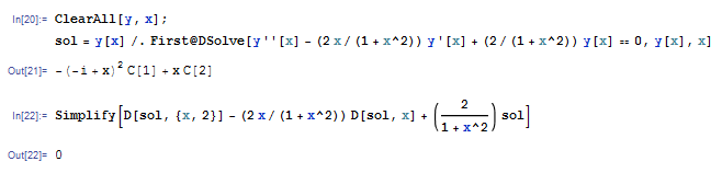
To verify the above solution, it is substituted back into the ODE \(y^{\prime \prime }-\frac{2x}{1+x^{2}}y^{\prime }+\frac{2}{1+x^{2}}y\) to check if the result is zero.\begin{align*} y^{\prime } & =c_{1}+c_{2}\left ( 2x\right ) \\ y^{\prime \prime } & =2c_{2} \end{align*}
Hence the ODE becomes\begin{align*} 0 & =y^{\prime \prime }-\frac{2x}{1+x^{2}}y^{\prime }+\frac{2}{1+x^{2}}y\\ & =\left ( 2c_{2}\right ) -\frac{2x}{1+x^{2}}\left ( c_{1}+c_{2}\left ( 2x\right ) \right ) +\frac{2}{1+x^{2}}\left ( c_{1}x+c_{2}\left ( x^{2}-1\right ) \right ) \\ & =2c_{2}-c_{1}\frac{2x}{1+x^{2}}-2xc_{2}\frac{2x}{1+x^{2}}+c_{1}x\frac{2}{1+x^{2}}+c_{2}\left ( x^{2}-1\right ) \frac{2}{1+x^{2}}\\ & =2c_{2}\left ( 1+x^{2}\right ) -2c_{1}x-4x^{2}c_{2}+2c_{1}x+2c_{2}\left ( x^{2}-1\right ) \\ & =2c_{2}+2c_{2}x^{2}-2c_{1}x-4x^{2}c_{2}+2c_{1}x+2c_{2}x^{2}-2c_{2}\\ & =4c_{2}x^{2}-4x^{2}c_{2}\\ & =0 \end{align*}
Verified OK.
Use the one solution indicated to find the complete solution. \(\left ( 2x-x^{2}\right ) y^{\prime \prime }+2\left ( x-1\right ) y^{\prime }-2y=0;y_{1}\left ( x\right ) =x-1\)
Solution:
The ODE can be written as \(y^{\prime \prime }+\frac{2\left ( x-1\right ) }{\left ( 2x-x^{2}\right ) }y^{\prime }-\frac{2}{\left ( 2x-x^{2}\right ) }y=0\). (assuming \(x\neq 0\)) Let the second solution of the ODE be \[ y_{2}=uy_{1}\] where \(u\left ( x\right ) \) is a function of \(x\) to be determined. The derivatives of \(y_{2}\) are now found and substituted back into the ODE to solve for \(u\).\begin{align} y_{2}^{\prime } & =u^{\prime }y_{1}+uy_{1}^{\prime }\tag{1}\\ y_{2}^{\prime \prime } & =u^{\prime \prime }y_{1}+u^{\prime }y_{1}^{\prime }+u^{\prime }y_{1}^{\prime }+uy_{1}^{\prime \prime } \tag{2} \end{align}
Since \(y_{2}\) is assumed to be a solution of the original ODE, then it satisfies it. Hence\begin{equation} y_{2}^{\prime \prime }+\frac{2\left ( x-1\right ) }{\left ( 2x-x^{2}\right ) }y_{2}^{\prime }-\frac{2}{\left ( 2x-x^{2}\right ) }y_{2}=0 \tag{3} \end{equation} Using Eqs. (1) and (2) into (3) gives\begin{align*} \left ( u^{\prime \prime }y_{1}+u^{\prime }y_{1}^{\prime }+u^{\prime }y_{1}^{\prime }+uy_{1}^{\prime \prime }\right ) +\frac{2\left ( x-1\right ) }{\left ( 2x-x^{2}\right ) }\left ( u^{\prime }y_{1}+uy_{1}^{\prime }\right ) -\frac{2}{\left ( 2x-x^{2}\right ) }uy_{1} & =0\\ u^{\prime \prime }y_{1}+u^{\prime }\left ( 2y_{1}^{\prime }+\frac{2\left ( x-1\right ) }{\left ( 2x-x^{2}\right ) }y_{1}\right ) +u\left ( y_{1}^{\prime \prime }+\frac{2\left ( x-1\right ) }{\left ( 2x-x^{2}\right ) }y_{1}^{\prime }-\frac{2}{\left ( 2x-x^{2}\right ) }y_{1}\right ) & =0 \end{align*}
But \(y_{1}\) is a solution of the ODE, hence the last term in the above vanishes resulting in\[ u^{\prime \prime }y_{1}+u^{\prime }\left ( 2y_{1}^{\prime }+\frac{2\left ( x-1\right ) }{\left ( 2x-x^{2}\right ) }y_{1}\right ) =0 \] But \(y_{1}=x-1\) and \(y_{1}^{\prime }=1\) hence the above becomes (assuming \(x\neq 1\))\begin{align*} u^{\prime \prime }\left ( x-1\right ) +u^{\prime }\left ( 2+\frac{2\left ( x-1\right ) }{\left ( 2x-x^{2}\right ) }\left ( x-1\right ) \right ) & =0\\ u^{\prime \prime }+u^{\prime }\left ( \frac{2}{\left ( x-1\right ) }+\frac{2\left ( x-1\right ) }{\left ( 2x-x^{2}\right ) }\right ) & =0\\ u^{\prime \prime }+u^{\prime }\left ( \frac{2\left ( 2x-x^{2}\right ) +2\left ( x-1\right ) \left ( x-1\right ) }{\left ( 2x-x^{2}\right ) \left ( x-1\right ) }\right ) & =0\\ u^{\prime \prime }+u^{\prime }\left ( \frac{4x-2x^{2}+2x^{2}+2-4x}{\left ( 2x-x^{2}\right ) \left ( x-1\right ) }\right ) & =0\\ u^{\prime \prime }+u^{\prime }\left ( \frac{2}{3x^{2}-2x-x^{3}}\right ) & =0 \end{align*}
Let \(u^{\prime }=v\), the above becomes\[ v^{\prime }+v\left ( \frac{2}{3x^{2}-2x-x^{3}}\right ) =0 \] This is now separable\[ \frac{v^{\prime }}{v}=-\left ( \frac{2}{3x^{2}-2x-x^{3}}\right ) \] Integrating both sides\[ \ln v=-2\int \frac{1}{3x^{2}-2x-x^{3}}dx+c_{1}\] Partial fraction decomposition on the integrand gives\begin{align*} \ln v & =-2\int \frac{1}{-2\left ( x-2\right ) }+\frac{1}{x-1}-\frac{1}{2x}dx+c_{1}\\ & =\int \frac{1}{\left ( x-2\right ) }-2\int \frac{1}{x-1}+\int \frac{1}{x}dx+c_{1}\\ & =\ln \left ( x-2\right ) -2\ln \left ( x-1\right ) +\ln x+c_{1} \end{align*}
Hence\begin{align*} v & =c_{1}e^{\ln \left ( x-2\right ) -2\ln \left ( x-1\right ) +\ln x}\\ & =c_{1}e^{\ln \left ( x-2\right ) }e^{-2\ln \left ( x-1\right ) }e^{\ln x}\\ & =c_{1}\frac{\left ( x-2\right ) x}{\left ( x-1\right ) ^{2}} \end{align*}
Since only one second solution \(y_{2}\) is needed, let \(c_{1}=1\).
Now that \(v\left ( x\right ) \) is found, then \(u\) is found by solving \begin{align*} u^{\prime } & =v\\ \frac{du}{dx} & =\frac{\left ( x-2\right ) x}{\left ( x-1\right ) ^{2}} \end{align*}
Hence\begin{align*} u & =\int \frac{x^{2}-2x}{\left ( x-1\right ) ^{2}}dx+c_{2}\\ & =x+\frac{1}{x-1}+c_{2} \end{align*}
Since only one second solution \(y_{2}\) is needed, let \(c_{2}=0\) hence \[ u=x+\frac{1}{x-1}\] Therefore, since \(y_{2}=uy_{1}\), and \(y_{1}=x-1\) then\begin{align*} y_{2} & =u\ y_{1}\\ & =\left ( x+\frac{1}{x-1}\right ) \left ( x-1\right ) \\ & =x\left ( x-1\right ) +1 \end{align*}
And finally, the general solution is\begin{align*} y & =c_{1}y_{1}+c_{2}y_{2}\\ & =c_{1}\left ( x-1\right ) +c_{2}\left ( x\left ( x-1\right ) +1\right ) \\ & =c_{1}\left ( x-1\right ) +c_{2}\left ( x^{2}-x+1\right ) \end{align*}
By letting \(c_{3}=(c_{1}-c_{2})\) the above can be simplified to \[ y(x)=c_{3}(x-1)+c_{2}x^{2}\] Or by constants renaming
\[ \fbox{$y(x)=c_1(x-1)+c_2x^2$}\] To verify the above solution, it is substituted back into the ODE \(y^{\prime \prime }+\frac{2\left ( x-1\right ) }{\left ( 2x-x^{2}\right ) }y^{\prime }-\frac{2}{\left ( 2x-x^{2}\right ) }y=0\) to check if the result is zero.\begin{align*} y^{\prime } & =c_{1}+2c_{2}x\\ y^{\prime \prime } & =2c_{2} \end{align*}
Hence the ODE becomes\begin{align*} 0 & =\left ( 2x-x^{2}\right ) y^{\prime \prime }+2\left ( x-1\right ) y^{\prime }-2y\\ & =\left ( 2x-x^{2}\right ) 2c_{2}+\left ( 2x-2\right ) \left ( c_{1}+2c_{2}x\right ) -2\left ( c_{1}(x-1)+c_{2}x^{2}\right ) \\ & =4c_{2}x-2c_{2}x^{2}+2c_{1}x+4c_{2}x^{2}-2c_{1}-4c_{2}x-2c_{1}x+2c_{1}-2c_{2}x^{2}\\ & =4c_{2}x+2c_{1}x-2c_{1}-4c_{2}x-2c_{1}x+2c_{1}\\ & =4c_{2}x-4c_{2}x\\ & =0 \end{align*}
Verified OK.
Problem 20, page 81. Solve \(x^{2}y^{\prime \prime }-9xy^{\prime }+24y=0;y\left ( 1\right ) =1;y^{\prime }\left ( 1\right ) =10\)
Solution:
This is Euler differential equation. Comparing to the standard form of Euler differential equation, which is given by\[ x^{2}y^{\prime \prime }+Axy^{\prime }+By=0 \] Where in the above \(y(x)\) is a function of \(x,\) shows that \(A=-9\) and \(B=24\).
Applying the transformation2 \(t=\ln (x)\) to the original ODE converts it to\begin{align} y^{\prime \prime }+(A-1)y^{\prime }+By & =0\nonumber \\ y^{\prime \prime }-10y^{\prime }+24y & =0 \tag{1} \end{align}
Where \(y(t)\) is now a function of \(t\) and not \(x\). This new ODE is solved for \(y(t)\). The solution is then converted back to be a function of \(x\).
Since Eq. (1) is now a constant coefficients ODE, direct application of characteristic roots method can be used. The roots of \(\lambda ^{2}-10\lambda +24=0\) are \(\lambda =\frac{-b\pm \sqrt{b^{2}-4ac}}{2a}=\frac{10\pm \sqrt{100-4\left ( 24\right ) }}{2}=\frac{10\pm \sqrt{4}}{2}=\frac{10\pm 2}{2}=\left \{ 6,4\right \} \). Therefore the solution to Eq. (1) is\[ y(t)=c_{1}e^{6t}+c_{2}e^{4t}\] The above solution is converted back to be a function of \(x\) using \(t=\ln (x).\)This results in \begin{align} y\left ( x\right ) & =c_{1}e^{6\ln \left ( x\right ) }+c_{2}e^{4\ln \left ( x\right ) }\nonumber \\ & =c_{1}x^{6}+c_{2}x^{4} \tag{2} \end{align}
This is valid for \(x>0\) and \(x<0\) but not for \(x=0\).\[ y^{\prime }=6c_{1}x^{5}+4c_{2}x^{3}\] At \(x=1\), \(y=1\), hence\[ 1=c_{1}+c_{2}\] At \(x=1,y^{\prime }\left ( 1\right ) =10\), hence\[ 10=6c_{1}+4c_{2}\] Hence \(c_{1}=1-c_{2}\), then \(10=6\left ( 1-c_{2}\right ) +4c_{2}\) or \(10=6-2c_{2}\) or \(c_{2}=-2\), hence \(c_{1}=1+2=3\), therefore the final solution is\[ \fbox{$y=3x^6-2x^4$}\]
Question:
To reduce the Euler equation to a linear equation, we use the substitution, \(z=\ln (x)\) to convert the equation from \(y(x)\) to an equation for \(y(z)\). If we use the operator notation3 \(D_{x}\equiv \frac{d}{dx}\) and \(D_{z}\equiv \frac{d}{dz}\) show that
Answer
\(\frac{dy}{dx}=\frac{dy}{dz}\frac{dz}{dx}\) but \(\frac{dz}{dx}=\frac{1}{x}\) hence \[ \frac{dy}{dx}=\frac{1}{x}\frac{dy}{dz}\] Using operator notation \[ D_{x}y=\frac{1}{x}D_{z}y \] or \[ xD_{x}y=D_{z}y \] Part 2
\(\frac{d^{2}y}{dx^{2}}=D_{x}^{2}y\) by definitions. This can be written as \[ \frac{d^{2}y}{dx^{2}}=\frac{d}{dx}\left ( \frac{dy}{dx}\right ) \] but from part(1) it was found that \(\frac{dy}{dx}=\frac{1}{x}\frac{dy}{dz}\), hence the above becomes\[ \frac{d^{2}y}{dx^{2}}=\frac{d}{dx}\left ( \frac{1}{x}\frac{dy}{dz}\right ) \] Applying chain rule\begin{align*} \frac{d^{2}y}{dx^{2}} & =\frac{-1}{x^{2}}\frac{dy}{dz}+\frac{1}{x}\frac{d}{dx}\frac{dy}{dz}\\ & =\frac{-1}{x^{2}}\frac{dy}{dz}+\frac{1}{x}\frac{d}{dz}\left ( \frac{dy}{dz}\right ) \left ( \frac{dz}{dx}\right ) \\ & =\frac{-1}{x^{2}}\frac{dy}{dz}+\frac{1}{x}\frac{d^{2}y}{dz^{2}}\left ( \frac{dz}{dx}\right ) \\ & =\frac{-1}{x^{2}}\frac{dy}{dz}+\frac{1}{x}\frac{d^{2}y}{dz^{2}}\left ( \frac{1}{x}\right ) \\ & =\frac{1}{x^{2}}\left ( \frac{d^{2}y}{dz^{2}}-\frac{dy}{dz}\right ) \end{align*}
Using operator notation \[ D_{x}^{2}y=\frac{1}{x^{2}}\left ( D_{z}^{2}y-D_{z}y\right ) \] or\[ x^{2}D_{x}^{2}y=D_{z}\left ( D_{z}-1\right ) y \]
\(\frac{d^{3}y}{dx^{3}}=D_{x}^{3}y\) by definitions. This can be written as \[ \frac{d^{3}y}{dx^{3}}=\frac{d}{dx}\left ( \frac{d^{2}y}{dx^{2}}\right ) \] but from part(2) it was found that \(\frac{d^{2}y}{dx^{2}}=\frac{1}{x^{2}}\left ( \frac{d^{2}y}{dz^{2}}-\frac{dy}{dz}\right ) \), hence the above becomes\[ \frac{d^{3}y}{dx^{3}}=\frac{d}{dx}\left ( \frac{1}{x^{2}}\left ( \frac{d^{2}y}{dz^{2}}-\frac{dy}{dz}\right ) \right ) \] Applying chain rule\begin{align*} \frac{d^{3}y}{dx^{3}} & =\frac{-2}{x^{3}}\left ( \frac{d^{2}y}{dz^{2}}-\frac{dy}{dz}\right ) +\frac{1}{x^{2}}\left ( \frac{d}{dx}\frac{d^{2}y}{dz^{2}}-\frac{d}{dx}\frac{dy}{dz}\right ) \\ & =\frac{-2}{x^{3}}\left ( \frac{d^{2}y}{dz^{2}}-\frac{dy}{dz}\right ) +\frac{1}{x^{2}}\left ( \frac{d}{dz}\frac{d^{2}y}{dz^{2}}\frac{dz}{dx}-\frac{d}{dz}\frac{dy}{dz}\frac{dz}{dx}\right ) \\ & =\frac{-2}{x^{3}}\left ( \frac{d^{2}y}{dz^{2}}-\frac{dy}{dz}\right ) +\frac{1}{x^{2}}\left ( \frac{d^{3}y}{dz^{3}}\frac{1}{x}-\frac{d^{2}y}{dz^{2}}\frac{1}{x}\right ) \\ & =\frac{-2}{x^{3}}\left ( \frac{d^{2}y}{dz^{2}}-\frac{dy}{dz}\right ) +\frac{1}{x^{3}}\left ( \frac{d^{3}y}{dz^{3}}-\frac{d^{2}y}{dz^{2}}\right ) \\ & =\frac{1}{x^{3}}\left [ \left ( -2\frac{d^{2}y}{dz^{2}}+2\frac{dy}{dz}\right ) +\left ( \frac{d^{3}y}{dz^{3}}-\frac{d^{2}y}{dz^{2}}\right ) \right ] \\ & =\frac{1}{x^{3}}\left [ \frac{d^{3}y}{dz^{3}}-3\frac{d^{2}y}{dz^{2}}+2\frac{dy}{dz}\right ] \end{align*}
Using operator notation \begin{align*} D_{x}^{3}y & =\frac{1}{x^{3}}\left ( D_{z}^{3}y-3D_{z}^{2}y+2D_{z}y\right ) \\ x^{3}D_{x}^{3}y & =\left ( D_{z}^{3}-3D_{z}^{2}+2D_{z}\right ) y \end{align*}
Writing the RHS as \(\left ( \lambda ^{3}-3\lambda ^{2}+2\lambda \right ) \), then it is seen it can be factored as \(\lambda \left ( \lambda ^{2}-3\lambda +2\right ) =\lambda \left ( \lambda -1\right ) \left ( \lambda -2\right ) \), hence the above can be written as\[ x^{3}D_{x}^{3}y=D_{z}\left ( D_{z}-1\right ) \left ( D_{z}-2\right ) y \]
Find the complete solution of \(x^{3}y^{\prime \prime \prime }+4x^{2}y^{\prime \prime }-5xy^{\prime }-15y=x^{4}\)
solution:
This is a Euler differential equation since it is of the form \(a_{n}x^{n}y^{\left ( n\right ) }+a_{n-1}x^{n-1}y^{\left ( n-1\right ) }+\cdots +a_{1}\frac{d}{dx}y+a_{0}y=f\left ( x\right ) \). Let \(z=\ln \left ( x\right ) \), or \(x=e^{z}\) to convert the equation from \(y(x)\) to an equation for \(Y(z)\). hence \(\frac{dz}{dx}=\frac{1}{x}\) and using results from problem 6 above summarized below\begin{align*} \frac{dy}{dx} & =\frac{1}{x}\frac{dY}{dz}\\ \frac{d^{2}y}{dx^{2}} & =\frac{1}{x^{2}}\left ( \frac{d^{2}Y}{dz^{2}}-\frac{dY}{dz}\right ) \\ \frac{d^{3}y}{dx^{3}} & =\frac{1}{x^{3}}\left [ \frac{d^{3}Y}{dz^{3}}-3\frac{d^{2}Y}{dz^{2}}+2\frac{dY}{dz}\right ] \end{align*}
The homogeneous part of the ODE is first solved. Substituting the above three relations into the ODE gives\[ x^{3}\frac{1}{x^{3}}\left [ \frac{d^{3}Y}{dz^{3}}-3\frac{d^{2}Y}{dz^{2}}+2\frac{dY}{dz}\right ] +4x^{2}\frac{1}{x^{2}}\left ( \frac{d^{2}Y}{dz^{2}}-\frac{dY}{dz}\right ) -5x\frac{1}{x}\frac{dY}{dz}-15Y=0 \] Where \(Y\) is function of \(z\) and \(y\) is the original function of \(x.\)The above becomes\begin{align*} \frac{d^{3}Y}{dz^{3}}-3\frac{d^{2}Y}{dz^{2}}+2\frac{dY}{dz}+4\left ( \frac{d^{2}Y}{dz^{2}}-\frac{dY}{dz}\right ) -5\frac{dY}{dz}-15Y & =0\\ \frac{d^{3}Y}{dz^{3}}+\frac{d^{2}Y}{dz^{2}}-7\frac{dY}{dz}-15Y & =0 \end{align*}
This is now a constant coefficient ODE, which can be solved directly using the characteristic roots method.\[ \lambda ^{3}+\lambda ^{2}-7\lambda -15=0 \] The roots are \(\left \{ 3,-2-i,-2+i\right \} \), hence the solution is\begin{align*} Y\left ( z\right ) & =c_{1}e^{3z}+c_{2}e^{\left ( -2-i\right ) z}+c_{3}e^{\left ( -2+i\right ) z}\\ & =c_{1}e^{3z}+c_{2}e^{\left ( -2-i\right ) z}+c_{3}e^{\left ( -2+i\right ) z}\\ & =c_{1}e^{3z}+c_{2}e^{-2z}e^{-iz}+c_{3}e^{-2z}e^{iz}\\ & =c_{1}e^{3z}+e^{-2z}\left ( c_{2}e^{-iz}+c_{3}e^{iz}\right ) \\ & =c_{1}e^{3z}+e^{-2z}\left ( c_{2}\left ( \cos z-i\sin z\right ) +c_{3}\left ( \cos z+i\sin z\right ) \right ) \\ & =c_{1}e^{3z}+e^{-2z}\left ( c_{2}\cos z-c_{2}i\sin z+c_{3}\cos z+c_{3}i\sin z\right ) \\ & =c_{1}e^{3z}+e^{-2z}\left ( \left ( c_{2}+c_{3}\right ) \cos z+\left ( c_{3}-c_{2}\right ) i\sin z\right ) \end{align*}
Let \(\left ( c_{2}+c_{3}\right ) \) be new constant \(c_{4}\) and \(\left ( c_{3}-c_{2}\right ) i\) new constant \(c_{5}\), hence\[ Y\left ( z\right ) =c_{1}e^{3z}+e^{-2z}\left ( c_{4}\cos z+c_{5}\sin z\right ) \] Converting back to \(x\) using \(z=\ln \left ( x\right ) \)\begin{align*} y\left ( x\right ) & =c_{1}e^{3\ln x}+e^{-2\ln x}\left ( c_{4}\cos \left ( \ln x\right ) +c_{5}\sin \left ( \ln x\right ) \right ) \\ & =c_{1}x^{3}+\frac{1}{x^{2}}\left ( c_{4}\cos \left ( \ln x\right ) +c_{5}\sin \left ( \ln x\right ) \right ) \end{align*}
The above is the homogeneous part of the solution. The particular solution is now found. Since the homogeneous solution has the following forms of solutions in it \(x^{3},\frac{1}{x^{2}}\cos \left ( \ln x\right ) ,\frac{1}{x^{2}}\sin \left ( \ln x\right ) \), then using variation of parameters, assume \[ y_{p}=u_{1}y_{1}+u_{2}y_{2}+u_{3}y_{3}\] where\begin{align*} y_{1} & =x^{3}\\ y_{2} & =\frac{1}{x^{2}}\cos \left ( \ln x\right ) \\ y_{3} & =\frac{1}{x^{2}}\sin \left ( \ln x\right ) \end{align*}
Therefore\begin{align*} u_{1} & =\int \frac{W_{1}\left ( x\right ) f\left ( x\right ) }{W\left ( x\right ) }dx\\ u_{2} & =\int \frac{W_{2}\left ( x\right ) f\left ( x\right ) }{W\left ( x\right ) }dx\\ u_{3} & =\int \frac{W_{3}\left ( x\right ) f\left ( x\right ) }{W\left ( x\right ) }dx \end{align*}
Where \(f\left ( x\right ) =x^{4}\) and\begin{align*} W\left ( x\right ) & =\begin{vmatrix} y_{1} & y_{2} & y_{3}\\ y_{1}^{\prime } & y_{2}^{\prime } & y_{3}^{\prime }\\ y_{1}^{\prime \prime } & y_{2}^{\prime \prime } & y_{3}^{\prime \prime }\end{vmatrix} \\ & \\ & =\begin{vmatrix} x^{3} & \frac{1}{x^{2}}\cos \left ( \ln x\right ) & \frac{1}{x^{2}}\sin \left ( \ln x\right ) \\ 3x^{2} & \frac{-2}{x^{3}}\cos \left ( \ln x\right ) -\frac{1}{x^{3}}\sin \left ( \ln x\right ) & \frac{-2}{x^{3}}\sin \left ( \ln x\right ) +\frac{1}{x^{3}}\cos \left ( \ln x\right ) \\ 6x & \frac{6}{x^{4}}\cos \left ( \ln x\right ) +\frac{2}{x^{4}}\sin \left ( \ln x\right ) +\frac{3}{x^{4}}\sin \left ( \ln x\right ) -\frac{1}{x^{4}}\cos \left ( \ln x\right ) & \frac{-6}{x^{4}}\sin \left ( \ln x\right ) -\frac{2}{x^{4}}\cos \left ( \ln x\right ) -\frac{3}{x^{4}}\cos \left ( \ln x\right ) +\frac{1}{x^{4}}\sin \left ( \ln x\right ) \end{vmatrix} \\ & =\frac{1}{x^{4}}\left ( 26\cos ^{2}\left ( \ln x\right ) +50\cos \left ( \ln x\right ) \sin \left ( \ln x\right ) +36\sin ^{2}\left ( \ln x\right ) \right ) \end{align*}
And \begin{align*} W_{1}\left ( x\right ) & =\left ( -1\right ) ^{3-1}W\left ( y_{2},y_{3}\right ) \\ W_{2}\left ( x\right ) & =\left ( -1\right ) ^{3-2}W\left ( y_{1},y_{3}\right ) \\ W_{3}\left ( x\right ) & =\left ( -1\right ) ^{3-3}W\left ( y_{1},y_{2}\right ) \end{align*}
Hence\begin{align*} W_{1}\left ( x\right ) & =\left ( -1\right ) ^{2}\begin{vmatrix} y_{2} & y_{3}\\ y_{2}^{\prime } & y_{3}^{\prime }\end{vmatrix} =\begin{vmatrix} \frac{1}{x^{2}}\cos \left ( \ln x\right ) & \frac{1}{x^{2}}\sin \left ( \ln x\right ) \\ \frac{-2}{x^{3}}\cos \left ( \ln x\right ) -\frac{1}{x^{3}}\sin \left ( \ln x\right ) & \frac{-2}{x^{3}}\sin \left ( \ln x\right ) +\frac{1}{x^{3}}\cos \left ( \ln x\right ) \end{vmatrix} \\ & =\frac{1}{x^{5}}\left ( \cos ^{2}\left ( \ln x\right ) +\sin ^{2}\left ( \ln x\right ) \right ) \\ & \\ W_{2}\left ( x\right ) & =\left ( -1\right ) ^{3-2}\begin{vmatrix} y_{1} & y_{3}\\ y_{1}^{\prime } & y_{3}^{\prime }\end{vmatrix} =-\begin{vmatrix} x^{3} & \frac{1}{x^{2}}\sin \left ( \ln x\right ) \\ 3x^{2} & \frac{-2}{x^{3}}\sin \left ( \ln x\right ) +\frac{1}{x^{3}}\cos \left ( \ln x\right ) \end{vmatrix} =5\sin \left ( \ln x\right ) -\cos \left ( \ln x\right ) \\ & \\ W_{3}\left ( x\right ) & =\left ( -1\right ) ^{3-3}\begin{vmatrix} x^{3} & \frac{1}{x^{2}}\cos \left ( \ln x\right ) \\ 3x^{2} & \frac{-2}{x^{3}}\cos \left ( \ln x\right ) -\frac{1}{x^{3}}\sin \left ( \ln x\right ) \end{vmatrix} =-5\cos \left ( \ln x\right ) -\sin \left ( \ln x\right ) \end{align*}
Hence4 \begin{align*} u_{1} & =\int \frac{W_{1}\left ( x\right ) }{W\left ( x\right ) }\frac{f\left ( x\right ) }{a_{0}}dx\\ & =\int \frac{\frac{1}{x^{5}}\left ( \cos ^{2}\left ( \ln x\right ) +\sin ^{2}\left ( \ln x\right ) \right ) }{\frac{1}{x^{4}}\left ( 26\cos ^{2}\left ( \ln x\right ) +50\cos \left ( \ln x\right ) \sin \left ( \ln x\right ) +36\sin ^{2}\left ( \ln x\right ) \right ) }xdx\\ & =\frac{x}{26} \end{align*}
And\begin{align*} u_{2} & =\int \frac{W_{2}\left ( x\right ) }{W\left ( x\right ) }\frac{f\left ( x\right ) }{a_{0}}dx\\ & =\int \frac{5\sin \left ( \ln x\right ) -\cos \left ( \ln x\right ) }{\frac{1}{x^{4}}\left ( 26\cos ^{2}\left ( \ln x\right ) +50\cos \left ( \ln x\right ) \sin \left ( \ln x\right ) +36\sin ^{2}\left ( \ln x\right ) \right ) }xdx\\ & =\frac{-11}{962}x^{6}\cos \left ( \ln \left ( x\right ) \right ) +\frac{29}{962}x^{6}\sin \left ( \ln x\right ) \end{align*}
and\begin{align*} u_{3} & =\int \frac{W_{3}\left ( x\right ) }{W\left ( x\right ) }\frac{f\left ( x\right ) }{a_{0}}dx\\ & =\int \frac{-5\cos \left ( \ln x\right ) -\sin \left ( \ln x\right ) }{\frac{1}{x^{4}}\left ( 26\cos ^{2}\left ( \ln x\right ) +50\cos \left ( \ln x\right ) \sin \left ( \ln x\right ) +36\sin ^{2}\left ( \ln x\right ) \right ) }xdx\\ & =\frac{-29}{962}x^{6}\cos \left ( \ln \left ( x\right ) \right ) -\frac{11}{962}x^{6}\sin \left ( \ln x\right ) \end{align*}
Hence \begin{align*} y_{p} & =u_{1}y_{1}+u_{2}y_{2}+u_{3}y_{3}\\ & =\frac{x}{26}x^{3}+\left ( \frac{-11}{962}x^{6}\cos \left ( \ln \left ( x\right ) \right ) +\frac{29}{962}x^{6}\sin \left ( \ln x\right ) \right ) \frac{1}{x^{2}}\cos \left ( \ln x\right ) +\left ( \frac{-29}{962}x^{6}\cos \left ( \ln \left ( x\right ) \right ) -\frac{11}{962}x^{6}\sin \left ( \ln x\right ) \right ) \frac{1}{x^{2}}\sin \left ( \ln x\right ) \end{align*}
The above reduces to\[ y_{p}=\frac{x^{4}}{37}\] Hence the final solution is\[ y=c_{1}x^{3}+c_{4}\frac{1}{x^{2}}\cos \left ( \ln x\right ) +c_{5}\frac{1}{x^{2}}\sin \left ( \ln x\right ) +\frac{x^{4}}{37}\]
The differential equation \(\frac{dy}{dx}+\left ( \frac{1}{x}-1\right ) y=\frac{e^{2x}}{x}\) has boundary condition \(y\left ( 1\right ) =b\). Find the only value of \(b\) for which \(y\left ( 0\right ) \) is finite.
Solution:
The complete solution is first found. The \(y_{h}\) is found first\[ \frac{dy}{dx}+\left ( \frac{1}{x}-1\right ) y=0 \] This is separable\begin{align*} \frac{dy}{y} & =\left ( 1-\frac{1}{x}\right ) dx\\ \ln y & =x-\ln x+c\\ y & =ce^{x-\ln x}\\ & =\frac{ce^{x}}{x} \end{align*}
For the particular solution, try \(y_{p}=A\frac{e^{2x}}{x}\), hence \(y_{p}^{\prime }=A\left ( \frac{-1}{x^{2}}e^{2x}+\frac{2}{x}e^{2x}\right ) \), and the ODE becomes\begin{align*} A\left ( \frac{-1}{x^{2}}e^{2x}+\frac{2}{x}e^{2x}\right ) +\left ( \frac{1}{x}-1\right ) A\frac{e^{2x}}{x} & =\frac{e^{2x}}{x}\\ \frac{-A}{x^{2}}e^{2x}+\frac{2A}{x}e^{2x}+\frac{A}{x}\frac{e^{2x}}{x}-A\frac{e^{2x}}{x} & =\frac{e^{2x}}{x}\\ \frac{2A}{x}e^{2x}-A\frac{e^{2x}}{x} & =\frac{e^{2x}}{x}\\ A\frac{e^{2x}}{x} & =\frac{e^{2x}}{x} \end{align*}
Hence \(A=1\) and the complete solution is\[ y=\frac{ce^{x}}{x}+\frac{e^{2x}}{x}\] At \(y\left ( 1\right ) \) the above becomes\begin{align*} b & =ce+e^{2}\\ & =ce\left ( 1+e\right ) \end{align*}
Hence \[ c=\frac{b}{e\left ( 1+e\right ) }\] Therefore the solution is\begin{align*} y & =\frac{b}{e\left ( 1+e\right ) }\frac{e^{x}}{x}+\frac{e^{2x}}{x}\\ & =\frac{1}{x}\left ( \frac{b}{1+e}e^{x-1}+e^{2x}\right ) \end{align*}
Now at \(x=0\) the solution is required to be finite.\begin{align*} \lim _{x\rightarrow 0}y\left ( x\right ) & =\lim _{x\rightarrow 0}\frac{1}{x}\lim _{x\rightarrow 0}\left ( \frac{b}{1+e}e^{x-1}+e^{2x}\right ) \\ & =\lim _{x\rightarrow 0}\frac{1}{x}\left ( \frac{b}{1+e}e^{-1}+1\right ) \\ & =\lim _{x\rightarrow 0}\frac{1}{x}\left ( \frac{b}{e+e^{2}}+1\right ) \\ & =\lim _{x\rightarrow 0}\frac{1}{x}\left ( \frac{b+e+e^{2}}{e+e^{2}}\right ) \end{align*}
But \(e+e^{2}=k=\) \(10.\,\allowbreak 107\), a known constant, hence the above\[ \lim _{x\rightarrow 0}y\left ( x\right ) =\frac{1}{k}\lim _{x\rightarrow 0}\frac{1}{x}\left ( b+k\right ) \] If \(b+k=x_{0}=0\), then \(\lim _{x\rightarrow 0}\frac{b+k}{x}\rightarrow 0\), since \(\lim _{x\rightarrow 0}\frac{0}{x}=0\), therefore\[ b=-k \] Hence \[ b=-10.107 \] Is the only value.