
Nonlinear Eq, reducible to first order.
Find the general solution to \(y^{\prime \prime }=\left ( 1+\left ( y^{\prime }\right ) ^{2}\right ) ^{\frac{3}{2}}\)
This is non-linear, second order differential equation. Since \(x\) does not appear explicitly, let \(u=y^{\prime }\), then \(u^{\prime }=y^{\prime \prime }\) and the above differential equation becomes\[ u^{\prime }=\left ( 1+u^{2}\right ) ^{\frac{3}{2}}\] The above is now separable and solved for \(u\)\begin{align} \frac{du}{\left ( 1+u^{2}\right ) ^{\frac{3}{2}}} & =dx\nonumber \\ \frac{u}{\sqrt{1+u^{2}}} & =x+C\nonumber \end{align}
The above is solved explicitly for \(u\)\begin{align*} \frac{u^{2}}{1+u^{2}} & =\left ( x+C\right ) ^{2}\\ u^{2} & =\left ( 1+u^{2}\right ) \left ( x+C\right ) ^{2}\\ u^{2}-u^{2}\left ( x+C\right ) ^{2} & =\left ( x+C\right ) ^{2}\\ u^{2} & =\frac{\left ( x+C\right ) ^{2}}{1-\left ( x+C\right ) ^{2}}\\ u & =\pm \sqrt{\frac{\left ( x+C\right ) ^{2}}{1-\left ( x+C\right ) ^{2}}}=\pm \frac{\left ( x+C\right ) }{\sqrt{1-\left ( x+C\right ) ^{2}}} \end{align*}
Since \(u=y^{\prime }\) therefore\[ y^{\prime }=\pm \frac{\left ( x+C\right ) }{\sqrt{1-\left ( x+C\right ) ^{2}}}\] This is separable, hence the solution is\begin{align*} y\left ( x\right ) & =\pm \int \frac{\left ( x+C\right ) }{\sqrt{1-\left ( x+C\right ) ^{2}}}+C_{2}\\ & =\pm \sqrt{1-\left ( x+C\right ) ^{2}}+C_{2}\\ & =\pm \sqrt{1-x^{2}-2xC+C^{2}}+C_{2} \end{align*}
Find general solution to \(yy^{\prime \prime }=y^{2}y^{\prime }+\left ( y^{\prime }\right ) ^{2}\)
Solution: This is non-linear, second order differential equation.\begin{align*} y\frac{d^{2}y}{dx^{2}} & =y^{2}\frac{dy}{dx}+\left ( \frac{dy}{dx}\right ) ^{2}\\ \frac{d^{2}y}{dx^{2}} & =y\frac{dy}{dx}+\frac{1}{y}\left ( \frac{dy}{dx}\right ) ^{2} \end{align*}
Multiply by \(\frac{dx}{dy}\)\[ \frac{d^{2}y}{dx^{2}}\frac{dx}{dy}=y+\frac{1}{y}\frac{dy}{dx}\] Let \[ u\left ( y\right ) =\frac{dy}{dx}\] \(u\) here is function of \(y\).The differential equation becomes\begin{align*} \frac{du}{dx}\frac{1}{u} & =y+\frac{1}{y}u\\ \frac{du}{dx} & =yu+\frac{1}{y}u^{2} \end{align*}
Multiply by \(\frac{dx}{dy}\) and using that \(u=\frac{dy}{dx}\) the above reduces to\begin{align*} \frac{du}{dx}\frac{dx}{dy} & =yu\frac{dx}{dy}+\frac{u^{2}}{y}\frac{dx}{dy}\\ \frac{du}{dy} & =y+\frac{1}{y}\left ( \frac{dy}{dx}\right ) ^{2}\frac{dx}{dy}\\ & =y+\frac{1}{y}\left ( \frac{dy}{dx}\right ) \\ & =y+\frac{1}{y}u \end{align*}
Hence\[ \frac{du}{dy}-\frac{u}{y}=y \] This is solved for \(u\left ( y\right ) .\)The integrating factor is \(I_{f}=y^{-1}\) hence\begin{align*} d\left ( y^{-1}u\right ) & =y^{-1}y=1\\ y^{-1}u & =y+C_{1}\\ u & =y^{2}+C_{1}y \end{align*}
But \(u=\frac{dy}{dx}\) hence\begin{align*} \frac{dy}{dx} & =y^{2}+C_{1}y\\ \frac{dy}{dx}-y^{2}-C_{1}y & =0 \end{align*}
This is first order non-linear ODE. It is separable, hence\[ \frac{dy}{\left ( y^{2}+C_{1}y\right ) }=dx \] Applying partial fractions to the LHS gives\[ \frac{dy}{C_{1}y}-\frac{1}{C_{1}}\frac{dy}{C_{1}+y}=dx \] Integrating both sides now gives\begin{align*} \frac{1}{C_{1}}\ln y-\frac{1}{C_{1}}\ln \left ( y+C_{1}\right ) & =x+C_{2}\\ \ln y-\ln \left ( y+C_{1}\right ) & =C_{1}x+C_{3} \end{align*}
Where \(C_{3}=C_{1}C_{2}\)\begin{align*} \ln \frac{y}{y+C_{1}} & =C_{1}x+C_{3}\\ \frac{y}{y+C_{1}} & =C_{4}e^{C_{1}x}\\ y & =yC_{4}e^{C_{1}x}+C_{1}C_{4}e^{C_{1}x}\\ y-yC_{4}e^{C_{1}x} & =C_{1}C_{4}e^{C_{1}x}\\ y\left ( 1-C_{4}e^{C_{1}x}\right ) & =C_{1}C_{4}e^{C_{1}x}\\ y & =\frac{C_{1}C_{4}e^{C_{1}x}}{1-C_{4}e^{C_{1}x}} \end{align*}
First factor the equation using operator notation and then find the general solution\[ x^{2}y^{\prime \prime }+xy^{\prime }-y=0 \] Let \(D\equiv \frac{d}{dx}.\)The ODE can be written as\[ \left ( x^{2}D^{2}+xD-1\right ) y=0 \] The roots of the characteristic equation \(x^{2}\lambda ^{2}+x\lambda -1\) are \(m=\frac{-b\pm \sqrt{b^{2}-4ac}}{2a}=\frac{-x\pm \sqrt{x^{2}+4x^{2}}}{2x^{2}}=\frac{-x\pm x\sqrt{5}}{2x^{2}}=\frac{-1\pm \sqrt{5}}{2x}=\frac{-1}{2x}\pm \frac{\sqrt{5}}{2x}.\) Hence the roots are\begin{align*} m_{1} & =\frac{-1+\sqrt{5}}{2x}\\ m_{2} & =\frac{-1-\sqrt{5}}{2x} \end{align*}
The ODE becomes\[ \left ( D-m_{1}\right ) \left ( D-m_{2}\right ) y=0 \] Let \begin{equation} \left ( D-m_{2}\right ) y=v \tag{1} \end{equation} hence\[ \left ( D-m_{1}\right ) v=0 \] Solution of \(\left ( D-m\right ) v=0\) is solution of \(v^{\prime }-mv=0\) which is \(v\left ( x\right ) =Ae^{mx}\) hence the solution of the above becomes\begin{align*} v\left ( x\right ) & =Ae^{m_{1}x}\\ & =Ae^{\left ( \frac{-1+\sqrt{5}}{2x}\right ) x}\\ & =Ae^{\left ( \frac{-1+\sqrt{5}}{2}\right ) } \end{align*}
Hence \(v\left ( x\right ) \) is constant and does not depend on \(x.\) Let \(Ae^{\left ( \frac{-1+\sqrt{5}}{2}\right ) }=C_{1}\).Now from Eq. (1) \begin{align*} \left ( D-m_{2}\right ) y & =v=C_{1}\\ \frac{dy}{dx}-m_{2}y & =C_{1}\\ \frac{dy}{dx}+\frac{1+\sqrt{5}}{2x}y & =C_{1} \end{align*}
The solution to the homogenous equation is\begin{align*} \frac{dy_{h}}{dx}+\frac{1+\sqrt{5}}{2x}y & =0\\ \frac{dy_{h}}{y} & =-\frac{1+\sqrt{5}}{2x}dx\\ \ln y_{h} & =\frac{\left ( -1-\sqrt{5}\right ) }{2}\ln x+C\\ y_{h} & =C_{2}xe^{\frac{\left ( -1-\sqrt{5}\right ) }{2}}\\ y_{h} & =C_{3}x \end{align*}
For the particular solution, using the trial \(y_{p}=C\), hence \(\frac{dy_{p}}{dx}-m_{2}y_{p}=C_{1}\) or \(0-\frac{1+\sqrt{5}}{2x}C=C_{1}\), hence \(C_{1}=\frac{C_{4}}{x}\), so \[ y_{p}=\frac{C_{4}}{x}\] Therefore the general solution is\begin{align*} y & =y_{h}+y_{p}\\ & =C_{3}x+\frac{C_{4}}{x} \end{align*}
Where \(C_{4},C_{3}\) are constants that can be determined from initial or boundary conditions
\[ xy^{\prime \prime }+y^{\prime }=3x^{2}-x \] First the homogenous equation is solved. Let \(D\equiv \frac{d}{dx}\) hence\[ \left ( xD^{2}+D\right ) y_{h}=0 \] The roots of the characteristic equation \(\left ( x\lambda ^{2}+\lambda \right ) \) are \(m=\frac{-b\pm \sqrt{b^{2}-4ac}}{2a}=\frac{-1\pm \sqrt{1}}{2x}=\frac{-1\pm 1}{2x}\) hence the roots are\begin{align*} m_{1} & =\frac{-1+1}{2x}=0\\ m_{2} & =\frac{-1-1}{2x}=-\frac{1}{x} \end{align*}
Therefore \begin{align} \left ( D-m_{2}\right ) \left ( D-m_{1}\right ) y_{h} & =0\nonumber \\ \left ( D-m_{2}\right ) \left ( D\right ) y_{h} & =0 \tag{1} \end{align}
Let \begin{equation} \left ( D\right ) y_{h}=v \tag{2} \end{equation} Hence \begin{align*} \left ( D-m_{2}\right ) v\left ( x\right ) & =0\\ \frac{dv}{dx}-m_{2}v\left ( x\right ) & =0\\ \frac{dv}{v} & =m_{2}dx\\ \ln v & =\int \frac{-1}{x}dx+C\\ \ln v & =-\ln x+C \end{align*}
Hence\[ v\left ( x\right ) =\frac{C_{1}}{x}\] Where \(C_{1}\) is new constant. Eq. (2) becomes\begin{align*} \left ( D\right ) y_{h} & =v=\frac{C_{1}}{x}\\ y_{h}^{\prime } & =\frac{C_{1}}{x}\\ dy_{h} & =\frac{C_{1}}{x}dx\\ y_{h} & =C_{1}\ln x+C_{2} \end{align*}
To find particular solution, let \[ y_{p}=ax^{3}+bx^{2}+cx+d \] and \(y_{p}^{\prime }=3ax^{2}+2bx+c\) and \(y_{p}^{\prime \prime }=6ax+2b\) hence the original ODE becomes\begin{align*} x\left ( 6ax+2b\right ) +\left ( 3ax^{2}+2bx+c\right ) & =3x^{2}-x\\ 9ax^{2}+4bx+c & =3x^{2}-x \end{align*}
Hence \(c=0\) and \(a=\frac{1}{3}\) and \(4b=-1\) or \(b=-\frac{1}{4}\), therefore \[ y_{p}=\frac{1}{3}x^{2}-\frac{1}{4}x \] And the full solution is\begin{align*} y & =y_{h}+y_{p}\\ & =C_{1}\ln x+C_{2}+\frac{1}{3}x^{2}-\frac{1}{4}x \end{align*}
Problem page 69, problem 8
Show that \(y_{1}\left ( x\right ) =x\) and \(y_{2}\left ( x\right ) =x^{2}\) are linearly independent solutions to \(x^{2}y^{\prime \prime }-2xy^{\prime }+2y=0\) on \(\left [ -1,1\right ] \) but that \(W\left ( 0\right ) =0\). Why does this not contradict theorem 2.3.1 in this interval?
Theorem 2.3: Wronskian test: Let \(y_{1},y_{2}\) be solutions of \(y^{\prime \prime }+p\left ( x\right ) y^{\prime }+q\left ( x\right ) y=0\) on the open interval \(I\), then the following is true
Answer:
First we show that \(y_{1},y_{2}\) are solutions to the ODE. Looking at \(y_{1}\), then \(y_{1}^{\prime }=1,y^{\prime \prime }=0\). Substituting into the ODE gives\[ -2x+2x=0 \] Hence \(y_{1}\) is a solution. Looking now at \(y_{2}\), then \(y_{2}^{\prime }=2x,y^{\prime \prime }=2\). Substituting into the ODE gives\[ 2x^{2}-4x^{2}+2x^{2}=0 \] Hence \(y_{2}\) is also a solution. Now we will show they are linearly independent. Let \[ ay_{1}+by_{2}=0 \] Where \(a,b\) are constants. If there are non-zero constants \(a,b\) that will make the above true, then \(y_{1},y_{2}\) are linearly dependent. Another way to say this, is that if and only if when \(a=b=0\) then the above is true, then \(y_{1},y_{2}\) are linearly independent.
Let us assume that for all \(x\) the following is true\[ ax+bx^{2}=0 \] Let \(x=1\), then \(a+b=0\). Let \(x=-1\) then \(b-a=0\). Solving for \(a,b\) from these two equations shows that \(2b=0\) or \(b=0\), hence \(a=0\). Therefore, for \(ay_{1}+by_{2}\) to be zero then \(a=b=0\). This shows that \(y_{1},y_{2}\) are linearly independent.
The above showed that \(y_{1},y_{2}\) are solutions to the ODE and that they are linearly independent functions. Now the Wronskian test is applied\[ W=\begin{vmatrix} y_{1} & y_{2}\\ y_{1}^{\prime } & y_{2}^{\prime }\end{vmatrix} =\begin{vmatrix} x & x^{2}\\ 1 & 2x \end{vmatrix} =2x^{2}-x^{2}=x^{2}\] At point \(0\) we see that \(W\left ( 0\right ) =0\). This seems like a conflict. But the Abel’s stronger statement applies only for solutions of an ODE, which says that for second order ODE, if \(y_{1},y_{2}\) are linearly independent solutions of the ODE, then \(W\) can not be zero at any point in the interval. However, there is no conflict in this case, since at \(x=0\) this statement does not even apply, as we see that when \(x=0\) the first and second terms of the ODE itself vanish and we no longer have an ODE in first place. At any other point \(x\), where the ODE remain in effect as stated, then \(W\left ( x\right ) \neq 0\), and hence there is no conflict.
Summary: To show that two functions are linearly independent on an interval, it is enough to show that the \(W\) is not zero on any one point in the interval. We do not need to check at each point. It is only when these two functions are also solutions of the ODE, then we need to check that \(W\) is not zero on each point in the interval, where the ODE is defined. In this problem, it happened that at \(x=0\) the ODE itself is not defined since \(a_{0}=0\) there.
Show that \(y_{1}\left ( x\right ) =3e^{2x}-1\) and \(y_{2}\left ( x\right ) =e^{-x}+2\) are solutions of \(yy^{\prime \prime }+2y^{\prime }-\left ( y^{\prime }\right ) ^{2}=0\) but neither \(2y_{1}\) nor \(y_{1}+y_{2}\) is a solution. Why does this not contradict theorem 2.2?
Theorem 2.2: Let \(y_{1},y_{2}\) be solutions of \(y^{\prime \prime }+p\left ( x\right ) y^{\prime }+q\left ( x\right ) y=0\) on interval \(I\), then any linear combination of these solutions is also a solution.
Solution
First we show that the \(y_{1\text{ }}\)and \(y_{2}\) are solutions. This is done by substitution into the ODE and checking for identity. Starting with \(y_{1}\)
\(y_{1}^{\prime }=6e^{2x},y_{1}^{\prime \prime }=12e^{2x}\), hence the ODE become \begin{align*} y_{1}y_{1}^{\prime \prime }+2y_{1}^{\prime }-\left ( y_{1}^{\prime }\right ) ^{2} & =\left ( 3e^{2x}-1\right ) \left ( 12e^{2x}\right ) +2\left ( 6e^{2x}\right ) -\left ( 6e^{2x}\right ) ^{2}\\ & =36e^{4x}-12e^{2x}+12e^{2x}-36e^{4x}\\ & =0 \end{align*}
This shows that \(y_{1}\) is a solution. Now for \(y_{2}\) we have \(y_{2}^{\prime }=-e^{-x},y_{2}^{\prime \prime }=e^{-x}\), hence the ODE become \begin{align*} y_{1}y_{1}^{\prime \prime }+2y_{1}^{\prime }-\left ( y_{1}^{\prime }\right ) ^{2} & =\left ( e^{-x}+2\right ) \left ( e^{-x}\right ) +2\left ( -e^{-x}\right ) -\left ( -e^{-x}\right ) ^{2}\\ & =e^{-2x}+2e^{-x}-2e^{-x}-e^{-2x}\\ & =0 \end{align*}
Therefore \(y_{2}\) is also a solution. now to Check if \(2y_{1}\) is a solution. Let \(y_{3}=2y_{1}=6e^{2x}-2\) hence \(y_{3}^{\prime }=12e^{2x}\) and \(y_{3}^{\prime \prime }=24e^{2x}\). Substitution into the ODE gives\begin{align*} y_{3}y_{3}^{\prime \prime }+2y_{3}^{\prime }-\left ( y_{3}^{\prime }\right ) ^{2} & =\left ( 6e^{2x}-2\right ) \left ( 24e^{2x}\right ) +2\left ( 12e^{2x}\right ) -\left ( 12e^{2x}\right ) ^{2}\\ & =144e^{4x}-48e^{2x}+24e^{2x}-144e^{4x}\\ & =-24e^{2x}\\ & \neq 0 \end{align*}
Hence \(y_{3}=2y_{1}\) is not a solution.
Now to check that \(y_{1}+y_{2}\) is a solution or not. Let \(y_{4}=y_{1}+y_{2}=3e^{2x}-1+e^{-x}+2=3e^{2x}+e^{-x}+1\,\), hence \(y_{4}^{\prime }=6e^{2x}-e^{-x}\) and \(y_{4}^{\prime \prime }=12e^{2x}+e^{-x}\), and substitution into the ODE gives\begin{align*} y_{4}y_{4}^{\prime \prime }+2y_{4}^{\prime }-\left ( y_{4}^{\prime }\right ) ^{2} & =\left ( 3e^{2x}+e^{-x}+1\right ) \left ( 12e^{2x}+e^{-x}\right ) +2\left ( 6e^{2x}-e^{-x}\right ) -\left ( 6e^{2x}-e^{-x}\right ) ^{2}\\ & =36e^{4x}+3e^{x}+12e^{x}+e^{-2x}+12e^{2x}+e^{-x}+12e^{2x}-2e^{-x}-36e^{4x}-e^{-2x}+12e^{x}\\ & =27e^{x}-e^{-x}+24e^{2x}\\ & \neq 0 \end{align*}
Hence \(y_{4}=y_{1}+y_{2}\) is not a solution.
Now to answer the question. Since the ODE given is not linear, and not of the form \(y^{\prime \prime }+p\left ( x\right ) y^{\prime }+q\left ( x\right ) y=0\), then we need to check first that when using the solution \(2y_{1}\) or \(y_{1}+y_{2}\), the ODE remains of the same form shown above for these to be also solutions.
Let us try \(2y_{1}\) and substituting this into the ODE. This results in\begin{align*} yy^{\prime \prime }+2y^{\prime }-\left ( y^{\prime }\right ) ^{2} & =0\\ \left ( 2y_{1}\right ) \left ( 2y_{1}\right ) ^{\prime \prime }+2\left ( 2y_{1}\right ) ^{\prime }-\left [ \left ( 2y_{1}\right ) ^{\prime }\right ] ^{2} & =0\\ \left ( 2y_{1}\right ) 2y_{1}^{\prime \prime }+2\left ( 2y_{1}^{\prime }\right ) -\left ( 2y_{1}^{\prime }\right ) ^{2} & =0\\ 4y_{1}y_{1}^{\prime \prime }+4y_{1}^{\prime }-4\left ( y_{1}^{\prime }\right ) ^{2} & =0 \end{align*}
Dividing by \(4\)\[ y_{1}y_{1}^{\prime \prime }+y_{1}^{\prime }-\left ( y_{1}^{\prime }\right ) ^{2}=0 \] Comparing this with the original ODE, we see it is not the same ODE. The second term was \(2y^{\prime }\) and now it is \(y_{1}^{\prime }\). Hence \(2y_{1}\) is not a solution. The reason is due to the nonlinearity of the ODE, the theorem did not apply to it.
Checking now for the second trial solution \(y_{1}+y_{2}\) and substituting this into the ODE\begin{align*} yy^{\prime \prime }+2y^{\prime }-\left ( y^{\prime }\right ) ^{2} & =0\\ \left ( y_{1}+y_{2}\right ) \left ( y_{1}+y_{2}\right ) ^{\prime \prime }+2\left ( y_{1}+y_{2}\right ) ^{\prime }-\left [ \left ( y_{1}+y_{2}\right ) ^{\prime }\right ] ^{2} & =0\\ \left ( y_{1}+y_{2}\right ) \left ( y_{1}^{\prime \prime }+y_{2}^{\prime \prime }\right ) +2\left ( y_{1}^{\prime }+y_{2}^{\prime }\right ) -\left ( y_{1}^{\prime }+y_{2}^{\prime }\right ) ^{2} & =0\\ \left ( y_{1}+y_{2}\right ) \left ( y_{1}^{\prime \prime }+y_{2}^{\prime \prime }\right ) +2\left ( y_{1}^{\prime }+y_{2}^{\prime }\right ) -\left ( y_{1}^{\prime }\right ) ^{2}-\left ( y_{2}^{\prime }\right ) ^{2}-2y_{1}^{\prime }y_{2}^{\prime } & =0\\ \left ( y_{1}y_{1}^{\prime \prime }+y_{1}y_{2}^{\prime \prime }\right ) +\left ( y_{2}y_{1}^{\prime \prime }+y_{2}y_{2}^{\prime \prime }\right ) +2y_{1}^{\prime }+2y_{2}^{\prime }-\left ( y_{1}^{\prime }\right ) ^{2}-\left ( y_{2}^{\prime }\right ) ^{2}-2y_{1}^{\prime }y_{2}^{\prime } & =0\\ \left [ y_{1}y_{1}^{\prime \prime }+2y_{1}^{\prime }-\left ( y_{1}^{\prime }\right ) ^{2}\right ] +\left [ y_{2}y_{2}^{\prime \prime }+2y_{2}^{\prime }-\left ( y_{2}^{\prime }\right ) ^{2}\right ] +y_{1}y_{2}^{\prime \prime }+y_{2}y_{1}^{\prime \prime }-2y_{1}^{\prime }y_{2}^{\prime } & =0 \end{align*}
The terms in square brackets are zero, since they are solutions of the ODE and hence vanish, hence the above reduces to\[ y_{1}y_{2}^{\prime \prime }+y_{2}y_{1}^{\prime \prime }-2y_{1}^{\prime }y_{2}^{\prime }=0 \] This is not the same ODE we started with. For \(y_{3}=y_{1}+y_{2}\) to be a solution, the ODE obtain \(y_{3}y_{3}^{\prime \prime }+2y_{3}^{\prime }-\left ( y_{3}^{\prime }\right ) ^{2}=0\). The reason is due to the nonlinearity of the ODE.
Solve the IC problem \(\left ( D^{3}-6D^{2}+11D-6\right ) y=0\) with IC \(y=y^{\prime }=0\) and \(y^{\prime \prime }=2\) when \(x=0\)
We need to factor the characteristic equation \(\lambda ^{3}-6\lambda ^{2}+11\lambda -6=0.\) Guessing a root, we see that \(\lambda =2\) is a root. Long division gives \(\frac{\lambda ^{3}-6\lambda ^{2}+11\lambda -6}{\lambda -2}=\) \(\lambda ^{2}-4\lambda +3\), hence the characteristic equation is \(\left ( \lambda ^{2}-4\lambda +3\right ) \left ( \lambda -2\right ) \). Now we factor the quadratic giving the final answer of \(\left ( \lambda -1\right ) \left ( \lambda -3\right ) \left ( \lambda -2\right ) \). The ODE is now written as\[ \left ( D-1\right ) \left ( D-3\right ) \left ( D-2\right ) y=0 \] Let \(\left ( D-2\right ) y=v\) then\[ \left ( D-1\right ) \left ( D-3\right ) v=0 \] Let \(\left ( D-3\right ) v=u\) then\begin{align*} \left ( D-1\right ) u & =0\\ u^{\prime }-u & =0\\ \frac{du}{dx} & =u\left ( x\right ) \\ \ln u & =x+c_{1}\\ u & =c_{1}e^{x} \end{align*}
Backtracking to the previous ODE \begin{align*} \left ( D-3\right ) v & =u\\ \frac{dv}{dx}-3v & =c_{1}e^{x} \end{align*}
Integrating factor is \(I_{f}=e^{-3x}\) hence\begin{align*} \frac{d}{dx}\left ( I_{f}v\right ) & =I_{f}c_{1}e^{x}\\ I_{f}v & =\int I_{f}c_{1}e^{x}dx+c_{2}\\ & =c_{1}\int e^{-2x}dx+c_{2}\\ & =c_{1}\left ( \frac{-1}{2}e^{-2x}\right ) +c_{2}\\ v & =\frac{-c_{1}}{2e^{-3x}}e^{-2x}+\frac{c_{2}}{e^{-3x}}\\ & =\frac{-c_{1}}{2}e^{x}+c_{2}e^{3x} \end{align*}
Now backtracking to the first ODE\begin{align*} \left ( D-2\right ) y & =v\\ \frac{dy}{dx}-2y & =\frac{-c_{1}}{2}e^{x}+c_{2}e^{3x} \end{align*}
Integrating factor is \(I_{f}=e^{-2x}\) hence\begin{align*} \frac{d}{dx}\left ( I_{f}y\right ) & =I_{f}\left ( \frac{-c_{1}}{2}e^{x}+c_{2}e^{3x}\right ) \\ e^{-2x}y & =\int e^{-2x}\left ( \frac{-c_{1}}{2}e^{x}+c_{2}e^{3x}\right ) dx+c_{3}\\ & =\int \left ( \frac{-c_{1}}{2}e^{-x}+c_{2}e^{x}\right ) dx+c_{3}\\ & =\frac{c_{1}}{2}e^{-x}+c_{2}e^{x}+c_{3}\\ y & =\frac{c_{1}}{2}e^{x}+c_{2}e^{3x}+c_{3}e^{2x} \end{align*}
or letting \(\frac{c_{1}}{2}=c_{1}\) (new constant) then\[ y\left ( x\right ) =c_{1}e^{x}+c_{2}e^{3x}+c_{3}e^{2x}\] Now the constants are found from IC. \(y=y^{\prime }=0\) and \(y^{\prime \prime }=2\)
When \(x=0\) then \(y=0\), hence \begin{equation} 0=c_{1}+c_{2}+c_{3} \tag{1} \end{equation} Taking derivative, then\[ y^{\prime }\left ( x\right ) =c_{1}e^{x}+3c_{2}e^{3x}+2c_{3}e^{2x}\] Hence\begin{equation} 0=c_{1}+3c_{2}+2c_{3} \tag{2} \end{equation} Taking derivative again\[ y^{\prime \prime }\left ( x\right ) =c_{1}e^{x}+9c_{2}e^{3x}+4c_{3}e^{2x}\] At \(x=0\)\begin{equation} 2=c_{1}+9c_{2}+4c_{3} \tag{3} \end{equation} Solving Eqs. (1),(2),(3) for the constants gives \(c_{1}=1,c_{2}=1,c_{3}=-2\). The final solution is\[ y\left ( x\right ) =e^{x}+e^{3x}-2e^{2x}\]
Solve the IC problem \(8y^{\prime \prime \prime }-4y^{\prime \prime }+6y^{\prime }+5y=0\) with IC \(y=0,y^{\prime \prime }=y^{\prime }=1\) when \(x=0\)
Solution:
Writing the ODE as \(\left ( 8D^{3}-4D^{2}+6D+5\right ) y=0\). The first step is to factor the characteristic equation \(8\lambda ^{3}-4\lambda ^{2}+6\lambda +5=0.\)
By guessing an initial root as \(\lambda =-\frac{1}{2}\) with some trials, now performing long Division to reduce it to a quadratic and then applying the quadratic equation to obtain the remaining two roots. Hence\(\frac{8\lambda ^{3}-4\lambda ^{2}+6\lambda +5}{\lambda +\frac{1}{2}}=8\lambda ^{2}-8\lambda +10\).
The characteristic equation now becomes \(\left ( \lambda +\frac{1}{2}\right ) \left ( 8\lambda ^{2}-8\lambda +10\right ) \). Factoring the quadratic gives \(\frac{-b\pm \sqrt{b^{2}-4ac}}{2a}=\frac{8\pm \sqrt{64-4\left ( 8\right ) \left ( 10\right ) }}{16}=\frac{8\pm \sqrt{64-320}}{16}=\frac{8\pm 16i}{16}=\frac{1\pm 2i}{2}.\) This means the roots are \(\frac{1}{2}\pm i\). Hence the ODE becomes\[ \left ( D-\left ( \frac{1}{2}+i\right ) \right ) \left ( D-\left ( \frac{1}{2}-i\right ) \right ) \left ( D+\frac{1}{2}\right ) y=0 \] Let \(\left ( D+\frac{1}{2}\right ) y=v\) The ODE becomes\[ \left ( D-\left ( \frac{1}{2}+i\right ) \right ) \left ( D-\left ( \frac{1}{2}-i\right ) \right ) v=0 \] Let \(\left ( D-\left ( \frac{1}{2}-i\right ) \right ) v=u.\) The ODE becomes\begin{align*} \left ( D-\left ( \frac{1}{2}+i\right ) \right ) u & =0\\ \frac{du}{dx}-\left ( \frac{1}{2}+i\right ) u & =0 \end{align*}
This is separable with solution \(u=c_{1}e^{\left ( \frac{1}{2}+i\right ) x}\) backtracking to the previous ODE and solving\begin{align*} \left ( D-\left ( \frac{1}{2}-i\right ) \right ) v & =c_{1}e^{\left ( \frac{1}{2}+i\right ) x}\\ \frac{dv}{dx}-\left ( \frac{1}{2}-i\right ) v & =c_{1}e^{\left ( \frac{1}{2}+i\right ) x} \end{align*}
Integrating factor is \(I_{f}=e^{-\left ( \frac{1}{2}-i\right ) x}\) hence\begin{align*} \frac{d}{dx}\left ( I_{f}v\right ) & =I_{f}c_{1}e^{\left ( \frac{1}{2}+i\right ) x}\\ ve^{-\left ( \frac{1}{2}-i\right ) x} & =\int c_{1}e^{-\left ( \frac{1}{2}-i\right ) x}e^{\left ( \frac{1}{2}+i\right ) x}dx+c_{2}\\ & =c_{1}\int e^{\left [ -\left ( \frac{1}{2}-i\right ) +\left ( \frac{1}{2}+i\right ) \right ] x}dx+c_{2}\\ & =c_{1}\int e^{2ix}dx+c_{2}\\ & =c_{1}\frac{e^{2ix}}{2}+c_{2} \end{align*}
Therefore\begin{align*} v\left ( x\right ) & =c_{1}\frac{e^{2ix}}{2}e^{\left ( \frac{1}{2}-i\right ) x}+c_{2}e^{\left ( \frac{1}{2}-i\right ) x}\\ & =c_{1}e^{\left ( i+\frac{1}{2}\right ) x}+c_{2}e^{\left ( -i+\frac{1}{2}\right ) x} \end{align*}
Where \(c_{1}=\frac{c_{1}}{2}\). Backtracking to the first ODE, we now solve\begin{align*} \left ( D+\frac{1}{2}\right ) y & =v\\ \frac{dy}{dx}+\frac{1}{2}y & =c_{1}e^{\left ( i+\frac{1}{2}\right ) x}+c_{2}e^{\left ( -i+\frac{1}{2}\right ) x} \end{align*}
The integrating factor is \(e^{\frac{1}{2}x}\) hence\begin{align*} \frac{d}{dx}\left ( I_{f}y\right ) & =I_{f}\left ( c_{1}e^{\left ( i+\frac{1}{2}\right ) x}+c_{2}e^{\left ( -i+\frac{1}{2}\right ) x}\right ) \\ I_{f}y & =\int e^{\frac{1}{2}x}\left ( c_{1}e^{\left ( i+\frac{1}{2}\right ) x}+c_{2}e^{\left ( -i+\frac{1}{2}\right ) x}\right ) dx+c_{3}\\ & =\int c_{1}e^{\left ( i+1\right ) x}+c_{2}e^{\left ( -i+1\right ) x}dx+c_{3}\\ & =c_{1}\frac{e^{\left ( 1+i\right ) x}}{1+i}+c_{2}\frac{e^{\left ( 1-i\right ) x}}{1-i}+c_{3} \end{align*}
Therefore\begin{align*} y & =c_{1}\frac{e^{\left ( 1+i\right ) x}}{1+i}e^{\frac{-1}{2}x}+c_{2}\frac{e^{\left ( 1-i\right ) x}}{1-i}e^{\frac{-1}{2}x}+c_{3}e^{\frac{-1}{2}x}\\ & =e^{\frac{1}{2}x}\left ( c_{1}\frac{e^{ix}}{1+i}+c_{2}\frac{e^{-ix}}{1-i}\right ) +c_{3}e^{\frac{-1}{2}x} \end{align*}
But \(e^{ix}=\cos x+i\sin x\) and \(e^{-ix}=\cos x-i\sin x\), hence combining the above gives\begin{align*} y & =e^{\frac{1}{2}x}\left ( c_{1}\frac{\cos x+i\sin x}{1+i}+c_{2}\frac{\cos x-i\sin x}{1-i}\right ) +c_{3}e^{\frac{-1}{2}x}\\ & =e^{\frac{1}{2}x}\left ( \frac{c_{1}\left ( 1-i\right ) \left ( \cos x+i\sin x\right ) +c_{2}\left ( 1+i\right ) \left ( \cos x-i\sin x\right ) }{\left ( 1+i\right ) \left ( 1-i\right ) }\right ) +c_{3}e^{\frac{-1}{2}x}\\ & =e^{\frac{1}{2}x}\left ( \frac{c_{1}\left ( \cos x+i\sin x-i\left ( \cos x+i\sin x\right ) \right ) +c_{2}\left ( \cos x-i\sin x+i\left ( \cos x-i\sin x\right ) \right ) }{2}\right ) +c_{3}e^{\frac{-1}{2}x}\\ & =e^{\frac{1}{2}x}\left ( \frac{c_{1}\left ( \cos x+i\sin x-i\cos x+\sin x\right ) +c_{2}\left ( \cos x-i\sin x+i\cos x+\sin x\right ) }{2}\right ) +c_{3}e^{\frac{-1}{2}x}\\ & =e^{\frac{1}{2}x}\left ( \frac{\cos x\left ( c_{1}-ic_{1}+c_{2}+ic_{2}\right ) +\sin x\left ( c_{1}+ic_{1}-ic_{2}+c_{2}\right ) }{2}\right ) +c_{3}e^{\frac{-1}{2}x} \end{align*}
Let \(\frac{\left ( c_{1}-ic_{1}+c_{2}+ic_{2}\right ) }{2}=c_{4}\) and let \(\frac{\left ( c_{1}+ic_{1}-ic_{2}+c_{2}\right ) }{2}=c_{5}\), then the above reduces to\[ y=e^{\frac{1}{2}x}\left ( c_{4}\cos x+c_{5}\sin x\right ) +c_{3}e^{\frac{-1}{2}x}\] This is the general solution. \(c_{3},c_{4},c_{5}\) are found from IC. \(y=0,y^{\prime \prime }=y^{\prime }=1\)
When \(x=0\) and \(y=0\) \begin{equation} 0=c_{4}+c_{3} \tag{1} \end{equation} Now \[ y^{\prime }=\frac{1}{2}e^{\frac{1}{2}x}\left ( c_{4}\cos x+c_{5}\sin x\right ) +e^{\frac{1}{2}x}\left ( -c_{4}\sin x+c_{5}\cos x\right ) -\frac{1}{2}c_{3}e^{\frac{-1}{2}x}\] Hence at \(x=0\) \begin{equation} 1=\frac{1}{2}c_{4}+c_{5}-\frac{1}{2}c_{3} \tag{2} \end{equation} and \begin{align*} y^{\prime \prime } & =\frac{1}{4}e^{\frac{1}{2}x}\left ( c_{4}\cos x+c_{5}\sin x\right ) +\frac{1}{2}e^{\frac{1}{2}x}\left ( -c_{4}\sin x+c_{5}\cos x\right ) \\ & +\frac{1}{2}e^{\frac{1}{2}x}\left ( -c_{4}\sin x+c_{5}\cos x\right ) +\frac{1}{2}e^{\frac{1}{2}x}\left ( -c_{4}\cos x-c_{5}\sin x\right ) +\frac{1}{4}c_{3}e^{\frac{-1}{2}x} \end{align*}
Hence at \(x=0\) \begin{align} 1 & =\frac{1}{4}c_{4}+\frac{1}{2}c_{5}+\frac{1}{2}c_{5}-\frac{1}{2}c_{4}+\frac{1}{4}c_{3}\nonumber \\ & =\frac{1}{4}c_{3}-\frac{1}{4}c_{4}+c_{5} \tag{3} \end{align}
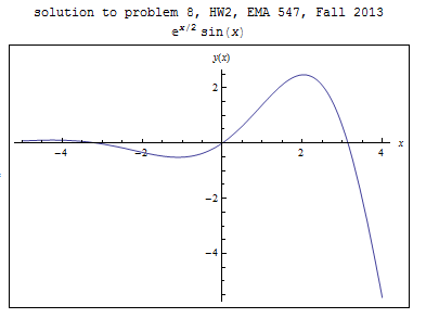
Solving Eqs. (1),(2),(3) for the constants gives \(c_{3}=0,c_{4}=0,c_{5}=1\), hence the solution is\[ y=e^{\frac{1}{2}x}\sin x \] A plot of the solution is
O’Neil. page 93, problem 16. Find general solution to \(y^{\prime \prime }-2y^{\prime }+y=3x+25\sin \left ( 3x\right ) \)
Write as \(\left ( D^{2}-2D+1\right ) y=3x+25\sin \left ( 3x\right ) \), where \(L\equiv D^{2}-2D+1=\left ( D-1\right ) \left ( D-1\right ) \). This will be solved two ways. The first using variation of parameters to obtain the particular solution, and the second by finding particular solution to each separate forcing function and adding.
\[ \left ( D-1\right ) \left ( D-1\right ) y_{h}=0 \] Let \(\left ( D-1\right ) y_{h}=v\), then\begin{align*} \left ( D-1\right ) v & =0\\ \frac{dv}{dx}-v & =0 \end{align*}
Solution is \(v=c_{1}e^{x}.\) We now backtrack and solve\begin{align*} \left ( D-1\right ) y_{h} & =v\\ \frac{dy_{1,h}}{dx}-y_{h} & =c_{1}e^{x} \end{align*}
Integrating factor is \(e^{-x}\) hence\begin{align*} \frac{d}{dx}\left ( I_{f}y_{h}\right ) & =e^{-x}\left ( c_{1}e^{x}\right ) \\ e^{-x}y_{h} & =c_{1}x+c_{2}\\ y_{h} & =c_{1}xe^{x}+c_{2}e^{x} \end{align*}
Hence \(y_{1}=xe^{x}\) and \(y_{2}=e^{x}\) are the two linearly independent solutions of the homogenous ODE. Let the particular solution be \[ y_{p}=u_{1}y_{1}+u_{2}y_{2}\] where \(u_{1}\left ( x\right ) ,u_{2}\left ( x\right ) \) are functions of \(x\) to be found. Hence \[ y_{p}^{\prime }=u_{1}^{\prime }y_{1}+u_{1}y_{1}^{\prime }+u_{2}^{\prime }y_{2}+u_{2}y_{2}^{\prime }\] and \[ y_{p}^{\prime \prime }=u_{1}^{\prime \prime }y_{1}+u_{1}^{\prime }y_{1}^{\prime }+u_{1}^{\prime }y_{1}^{\prime }+u_{1}y_{1}^{\prime \prime }+u_{2}^{\prime \prime }y_{2}+u_{2}^{\prime }y_{2}^{\prime }+u_{2}^{\prime }y_{2}^{\prime }+u_{2}y_{2}^{\prime \prime }\] Therefore, the ODE \(y_{p}^{\prime \prime }-2y_{p}^{\prime }+y_{p}=3x+25\sin \left ( 3x\right ) \) becomes

If \begin{equation} u_{1}^{\prime }y_{1}+u_{2}^{\prime }y_{2}=0 \tag{1} \end{equation} then the above becomes\begin{equation} \left ( u_{1}^{\prime }y_{1}^{\prime }+u_{2}^{\prime }y_{2}^{\prime }\right ) =f\left ( x\right ) =3x+25\sin \left ( 3x\right ) \tag{2} \end{equation} Hence we have two equations Eqs. (1),(2) to solve for \(u_{1},u_{2}\)\[ u_{1}=\int \frac{-y_{2}}{y_{1}y_{2}^{\prime }-y_{2}y_{1}^{\prime }}f\left ( x\right ) dx=\int \frac{-y_{2}}{W\left ( x\right ) }f\left ( x\right ) dx \] But\[ W\left ( x\right ) =\begin{vmatrix} y_{1} & y_{2}\\ y_{1}^{\prime } & y_{2}^{\prime }\end{vmatrix} =\begin{vmatrix} xe^{x} & e^{x}\\ e^{x}+xe^{x} & e^{x}\end{vmatrix} =xe^{2x}-\left ( e^{2x}+xe^{2x}\right ) =-e^{2x}\] Hence\begin{align*} u_{1} & =\int \frac{-e^{x}}{-e^{2x}}\left ( 3x+25\sin \left ( 3x\right ) \right ) dx\\ & =\int e^{-x}\left ( 3x+25\sin \left ( 3x\right ) \right ) dx\\ & =3\int xe^{-x}+25\int e^{-x}\sin \left ( 3x\right ) dx\\ & =e^{-x}\left ( -3-3x-\frac{15}{2}\cos \left ( 3x\right ) -\frac{5}{2}\sin \left ( 3x\right ) \right ) \end{align*}
and\begin{align*} u_{2} & =\int \frac{y_{1}}{W\left ( x\right ) }f\left ( x\right ) dx\\ & =\int \frac{xe^{x}}{-e^{2x}}\left ( 3x+25\sin \left ( 3x\right ) \right ) dx\\ & =-\int xe^{-x}\left ( 3x+25\sin \left ( 3x\right ) \right ) dx\\ & =-3\int x^{2}e^{-x}dx-25\int e^{-x}x\sin \left ( 3x\right ) dx\\ & =e^{-x}\left ( 6+6x+3x^{2}+\frac{3}{2}\cos 3x+\frac{15}{2}x\cos 3x-2\sin 3x+\frac{5}{2}x\sin 3x\right ) \end{align*}
Therefore \begin{align*} y_{p} & =u_{1}y_{1}+u_{2}y_{2}\\ & =e^{-x}\left [ -3-3x-\frac{15}{2}\cos \left ( 3x\right ) -\frac{5}{2}\sin \left ( 3x\right ) \right ] xe^{x}\\ & +\left ( e^{-x}\left ( 6+6x+3x^{2}+\frac{3}{2}\cos 3x+\frac{15}{2}x\cos 3x-2\sin 3x+\frac{5}{2}x\sin 3x\right ) \right ) e^{x}\\ & \\ & =-3x-3x^{2}-\frac{15}{2}x\cos \left ( 3x\right ) -\frac{5}{2}x\sin \left ( 3x\right ) +6+6x+3x^{2}+\frac{3}{2}\cos 3x+\frac{15}{2}x\cos 3x-2\sin 3x+\frac{5}{2}x\sin 3x\\ & =3x+\frac{3}{2}\cos 3x-2\sin 3x+6 \end{align*}
Hence the total solution is\begin{align*} y & =y_{h}+y_{p}\\ & =c_{1}xe^{x}+c_{2}e^{x}+3x+\frac{3}{2}\cos 3x-2\sin 3x+6 \end{align*}
This will be solved by breaking the forcing functions and solving for each separately and then adding the solutions at the end since the ODE is linear. Hence we will solve the following two ODE’s\begin{align*} y_{1}^{\prime \prime }-2y_{1}^{\prime }+y_{1} & =3x\\ y_{2}^{\prime \prime }-2y_{2}^{\prime }+y_{2} & =25\sin \left ( 3x\right ) \end{align*}
and the solution will be \(y=y_{1}+y_{2}\). Starting with the first one, we solve for the homogeneous and then for the particular.\[ \left ( D-1\right ) \left ( D-1\right ) y_{1,h}=0 \] Now we processed as before. Let \(\left ( D-1\right ) y_{1,h}=v\), then\begin{align*} \left ( D-1\right ) v & =0\\ \frac{dv}{dx}-v & =0 \end{align*}
Solution is \(v=c_{1}e^{x}.\) We now backtrack and solve\begin{align*} \left ( D-1\right ) y_{1,h} & =v\\ \frac{dy_{1,h}}{dx}-y_{1,h} & =c_{1}e^{x} \end{align*}
Integrating factor is \(e^{-x}\) hence\begin{align*} \frac{d}{dx}\left ( I_{f}y_{1,h}\right ) & =e^{-x}\left ( c_{1}e^{x}\right ) \\ e^{-x}y_{1,h} & =c_{1}x+c_{2}\\ y_{1,h} & =c_{1}xe^{x}+c_{2}e^{x} \end{align*}
Now we find the particular solution \(y_{1,p}\).
Let \(y_{1,p}=ax^{2}+bx+c\), hence \(y_{1,p}^{\prime }=2ax+b\) and \(y_{1,p}^{\prime \prime }=2a\), therefore the ODE becomes\begin{align*} 2a-2\left ( 2ax+b\right ) +ax^{2}+bx+c & =3x\\ x^{2}\left ( a\right ) +x\left ( -4a+b\right ) +2a-2b+c & =3x \end{align*}
Hence \(a=0\) and \(-2b+c=0\) and \(b=3\). Therefore \(c=6\) and the forcing function is \(y_{1,p}=3x+6\), hence\[ y_{1}=c_{1}xe^{x}+c_{2}e^{x}+3x+6 \] We now solve the second ode \[ y_{2}^{\prime \prime }-2y_{2}^{\prime }+y_{2}=25\sin \left ( 3x\right ) \] The homogenous solution is the same as above, \(y_{2,h}=c_{1}xe^{x}+c_{2}e^{x}\). Only the particular solution needs to be found again. Let \(y_{2,p}=A\sin 3x+B\cos 3x\), hence \(y_{2,p}^{\prime }=3A\cos 3x-3B\sin 3x\) and \(y_{2,p}^{\prime \prime }=-9A\sin 3x-9B\cos x\). The ODE becomes\begin{align*} -9A\sin 3x-9B\cos x-2\left ( 3A\cos 3x-3B\sin 3x\right ) +A\sin 3x+B\cos 3x & =25\sin \left ( 3x\right ) \\ \sin 3x\left ( -9A+6B+A\right ) +\cos 3x\left ( -9B-6A+B\right ) & =25\sin \left ( 3x\right ) \end{align*}
Therefore, \(\left ( -8A+6B\right ) =25\) and \(\left ( -8B-6A\right ) =0\), from the first equation \(A=\frac{6B-25}{8}\), and from the second \(-8B-6\frac{6B-25}{8}=0\) or \(-64B-36B+150=0\) or \(B=1.5\), hence \(A=\frac{9-25}{8}=-2\), therefore \[ y_{2,p}=-2\sin 3x+\frac{3}{2}\cos 3x \] And the general solution is\[ y=c_{1}xe^{x}+c_{2}e^{x}+3x+6-2\sin 3x+\frac{3}{2}\cos 3x \] This answer matches the answer obtained above using variation of parameters.
Find general solution \(y^{\left ( 4\right ) }+3y^{\prime \prime }-4y=\sinh \left ( x\right ) -\sin ^{2}x\)
First the homogenous solution is find using the operator method. Let \[ \left ( D^{4}+3D^{2}-4\right ) y=\sinh \left ( x\right ) -\sin ^{2}x \] The characteristic equation is \(\lambda ^{4}+3\lambda ^{2}-4=0\). Let \(\lambda ^{2}=u\), hence \(u^{2}-u-4=0\), and the roots are \(u=\left \{ 1,-4\right \} \). Hence when \(u=1,\lambda =\pm 1\) and when \(u=-4,\lambda =\pm 2i\), therefore we obtain the 4 roots as \(\left \{ 1,-1,2i,-2i\right \} \) and the factorization is\[ \left ( D-1\right ) \left ( D+1\right ) \left ( D-2i\right ) \left ( D+2i\right ) y=\sinh \left ( x\right ) -\sin ^{2}x \] Solving the homogenous part first.\[ \left ( D-1\right ) \left ( D+1\right ) \left ( D-2i\right ) \left ( D+2i\right ) y=0 \] Let \(\left ( D+2i\right ) y=v\), hence\[ \left ( D-1\right ) \left ( D+1\right ) \left ( D-2i\right ) v=0 \] Let \(\left ( D-2i\right ) v=u\) hence\[ \left ( D-1\right ) \left ( D+1\right ) u=0 \] Let \(\left ( D+1\right ) u=r\) hence\begin{align*} \left ( D-1\right ) r & =0\\ \frac{dr}{dx}-r & =0 \end{align*}
And the solution is \(r\left ( x\right ) =c_{1}e^{x}\), backtracking now we solve\begin{align*} \left ( D+1\right ) u & =c_{1}e^{x}\\ \frac{du}{dx}+u & =c_{1}e^{x} \end{align*}
Integration factor is \(e^{x}\), hence\begin{align*} \frac{d}{dx}\left ( e^{x}u\right ) & =e^{x}\left ( c_{1}e^{x}\right ) \\ e^{x}u & =c_{1}\int e^{2x}dx+c_{2}\\ & =c_{1}\frac{e^{2x}}{2}+c_{2} \end{align*}
Therefore\[ u=c_{1}\frac{e^{x}}{2}+c_{2}e^{-x}\] Let \(c_{1}=\frac{1}{2}c_{1}\), hence\[ u=c_{1}e^{x}+c_{2}e^{-x}\] Backtracking, we now solve \begin{align*} \left ( D-2i\right ) v & =u\\ \frac{dv}{dx}-2iv & =c_{1}e^{x}+c_{2}e^{-x} \end{align*}
Integration factor is \(e^{-2ix}\) hence\begin{align*} \frac{d}{dx}\left ( e^{-2ix}v\right ) & =e^{-2ix}\left ( c_{1}e^{x}+c_{2}e^{-x}\right ) \\ e^{-2ix}v & =\int e^{-2ix}\left ( c_{1}e^{x}+c_{2}e^{-x}\right ) dx+c_{3}\\ & =c_{1}\int e^{-2ix+x}dx+c_{2}\int e^{-2ix-x}dx+c_{3}\\ & =c_{1}\frac{e^{-2ix+x}}{-2i+1}+c_{2}\frac{e^{-2ix-x}}{-2i-1}+c_{3} \end{align*}
Hence\begin{align*} v & =e^{2ix}c_{1}\frac{e^{-2ix+x}}{-2i+1}+e^{2ix}c_{2}\frac{e^{-2ix-x}}{-2i-1}+e^{2ix}c_{3}\\ & =c_{1}\frac{e^{x}}{-2i+1}+c_{2}\frac{e^{-x}}{-2i-1}+e^{2ix}c_{3} \end{align*}
Now we backtrack one last time and solve for \(y_{h}\)\begin{align*} \left ( D+2i\right ) y_{h} & =v\\ \frac{dy_{h}}{dx}+2iy_{h} & =c_{1}\frac{e^{x}}{-2i+1}+c_{2}\frac{e^{-x}}{-2i-1}+e^{2ix}c_{3} \end{align*}
Integration factor is \(e^{2ix}\) hence\begin{align*} \frac{d}{dx}\left ( e^{2ix}y_{h}\right ) & =e^{2ix}\left ( c_{1}\frac{e^{x}}{-2i+1}+c_{2}\frac{e^{-x}}{-2i-1}+e^{2ix}c_{3}\right ) \\ e^{2ix}y_{h} & =\int e^{2ix}\left ( c_{1}\frac{e^{x}}{-2i+1}+c_{2}\frac{e^{-x}}{-2i-1}+e^{2ix}c_{3}\right ) dx+c_{4}\\ & =\frac{c_{1}}{-2i+1}\int e^{x+2ix}dx+\frac{c_{2}}{-2i-1}\int e^{-x+2ix}dx+\int e^{4ix}c_{3}dx+c_{4}\\ & =\frac{c_{1}}{-2i+1}\frac{e^{x+2ix}}{1+2i}-\frac{c_{2}}{-2i-1}\frac{e^{-x+2ix}}{-1+2i}+\frac{c_{3}}{4i}e^{4ix}+c_{4}\\ & =\frac{c_{1}}{5}e^{x+2ix}-\frac{c_{2}}{5}e^{-x+2ix}+\frac{c_{3}}{4i}e^{4ix}+c_{4} \end{align*}
Hence\begin{align*} y_{h} & =e^{-2ix}\left ( \frac{c_{1}}{5}e^{x+2ix}-\frac{c_{2}}{5}e^{-x+2ix}+\frac{c_{3}}{4i}e^{4ix}+c_{4}\right ) \\ & =\frac{c_{1}}{5}e^{x}-\frac{c_{2}}{5}e^{-x}+\frac{c_{3}}{4i}e^{2ix}+c_{4}e^{-2ix} \end{align*}
Let \(\frac{c_{1}}{5}=c_{1}\) and \(\frac{-c_{2}}{5}=c_{2}\) and \(\frac{-c_{3}}{4}=c_{3}\) the above simplifies to\begin{align*} y_{h} & =c_{1}e^{x}+c_{2}e^{-x}-c_{3}\frac{e^{2ix}}{i}+c_{4}e^{-2ix}\\ & =c_{1}e^{x}+c_{2}e^{-x}+c_{3}ie^{2ix}+c_{4}e^{-2ix} \end{align*}
Convert to trig using Euler’s we obtain\begin{align*} y_{h} & =c_{1}e^{x}+c_{2}e^{-x}+c_{3}i\left ( \cos 2x+i\sin 2x\right ) +c_{4}\left ( \cos 2x-i\sin 2x\right ) \\ & =c_{1}e^{x}+c_{2}e^{-x}+\cos \left ( 2x\right ) \left ( ic_{3}+c_{4}\right ) +\sin \left ( 2x\right ) \left ( -c_{3}-ic_{4}\right ) \end{align*}
Let \(\left ( ic_{3}+c_{4}\right ) =c_{5}\) and \(\left ( -c_{3}-ic_{4}\right ) =c_{6}\), new constants, hence\[ y_{h}=c_{1}e^{x}+c_{2}e^{-x}+c_{5}\cos \left ( 2x\right ) +c_{6}\sin \left ( 2x\right ) \]
To find the particular solution, using superposition. Since \(\left ( D^{4}+3D^{2}-4\right ) y=\sinh \left ( x\right ) -\sin ^{2}x\), we solve first for the first forcing function\[ \left ( D^{4}+3D^{2}-4\right ) y=\sinh \left ( x\right ) \] \(\sinh \left ( x\right ) \) can not be used for trail solution, as the homogeneous solution include \(e^{x}\) in it and \(\sinh \left ( x\right ) =-\frac{e^{-x}}{2}+\frac{e^{x}}{2}\). Therefore we will use \(Axe^{x}+Cxe^{-x}\) as trial solution. Hence \begin{align*} y_{p1} & =Ae^{x}+Bxe^{x}+Ce^{-x}+Dxe^{-x}\\ y_{p1}^{\prime } & =Ae^{x}+Be^{x}+Bxe^{x}-Ce^{-x}+De^{-x}-Dxe^{-x}\\ y_{p1}^{\prime \prime } & =Ae^{x}+Be^{x}+Be^{x}+Bxe^{x}+Ce^{-x}-De^{-x}-De^{-x}+Dxe^{-x}\\ & =Ae^{x}+2Be^{x}+Bxe^{x}+Ce^{-x}-2De^{-x}+Dxe^{-x}\\ y_{p1}^{\prime \prime \prime } & =Ae^{x}+2Be^{x}+Be^{x}+Bxe^{x}-Ce^{-x}+2De^{-x}+De^{-x}-Dxe^{-x}\\ & =Ae^{x}+3Be^{x}+Bxe^{x}-Ce^{-x}+3De^{-x}-Dxe^{-x}\\ y_{p1}^{\prime \prime \prime \prime } & =Ae^{x}+3Be^{x}+Be^{x}+Bxe^{x}+Ce^{-x}-3De^{-x}-De^{-x}+Dxe^{-x}\\ & =Ae^{x}+4Be^{x}+Bxe^{x}+Ce^{-x}-4De^{-x}+Dxe^{-x} \end{align*}
Therefore the ODE becomes, and using \(\frac{e^{x}}{2}-\frac{e^{-x}}{2}\) for \(\sinh \left ( x\right ) \)\begin{multline*} \left ( D^{4}+3D^{2}-4\right ) y_{p1}=\left ( Ae^{x}+4Be^{x}+Bxe^{x}+Ce^{-x}-4De^{-x}+Dxe^{-x}\right ) \\ +3\left ( Ae^{x}+2Be^{x}+Bxe^{x}+Ce^{-x}-2De^{-x}+Dxe^{-x}\right ) \\ -4\left ( Ae^{x}+Bxe^{x}+Ce^{-x}+Dxe^{-x}\right ) =\frac{e^{x}}{2}-\frac{e^{-x}}{2} \end{multline*} Hence, comparing coefficients \[ e^{x}\left ( A+4B+3A+6B-4A\right ) +e^{-x}\left ( C-4D+3C-6D-4C\right ) +xe^{x}\left ( B+3B-4B\right ) +xe^{-x}\left ( D+3D-4D\right ) =\frac{e^{x}}{2}-\frac{e^{-x}}{2}\] Hence \begin{align*} A+4B+3A+6B-4A & =\frac{1}{2}\\ C-4D+3C-6D-4C & =-\frac{1}{2} \end{align*}
Hence\begin{align*} 10B & =\frac{1}{2}\\ -10D & =-\frac{1}{2} \end{align*}
Hence\begin{align*} B & =\frac{1}{20}\\ D & =\frac{1}{20} \end{align*}
Therefore \[ y_{1p}=\frac{1}{20}xe^{x}+\frac{1}{20}xe^{-x}\] To find second particular solution,\[ \left ( D^{4}+3D^{2}-4\right ) y=-\sin ^{2}x \] Since \(\sin ^{2}x=\frac{1}{2}-\frac{1}{4}\left ( e^{-2ix}+e^{2ix}\right ) \) and the functions \(e^{\pm 2ix}\) are in the homogeneous solution, let the trial function be \(y_{p2}=a+bxe^{-2ix}+cxe^{2ix}.\) Plug-in this into the ODE and expanding gives\[ e^{-2ix}\left ( 32ib+16xb-12ib-4bx\right ) +e^{2ix}\left ( -32ic+16xc+12ic-12cx-4bx\right ) -4a=\frac{1}{2}-\frac{1}{4}\left ( e^{-2ix}+e^{2ix}\right ) \] This can be used to find \(y_{p2}\) (need to more time to work this out). The final solution will then be\begin{align*} y & =y_{h}+y_{p1}+y_{p2}\\ y_{h} & =c_{1}e^{x}+c_{2}e^{-x}+c_{5}\cos \left ( 2x\right ) +c_{6}\sin \left ( 2x\right ) +\frac{1}{20}xe^{x}+\frac{1}{20}xe^{-x}+y_{p2} \end{align*}
note:
I verified the solution using Mathematica. The homogeneous solution appears to be correct, but need to work more on the particular solution. Here is the result\[ y\left ( x\right ) =c_{1}e^{x}+c_{2}e^{-x}+c_{5}\cos \left ( 2x\right ) +c_{6}\sin \left ( 2x\right ) +y_{p}\] Where \(y_{p}\) was given as \(\frac{1}{800}e^{-x}\Delta \) where \begin{multline*} \Delta =-80e^{x}-20e^{2x}+40e^{2x}x+40x-20e^{x}\sin ^{2}(2x)+20e^{x}x\sin (2x)\\ +5e^{x}\sin (2x)\sin (4x)+10e^{x}\cos ^{3}(2x)-20e^{x}\cos ^{2}(2x)+\\ 16e^{x}\cos (2x)-32e^{x}\sin ^{2}(2x)\sinh (x)-32e^{x}\cos ^{2}(2x)\sinh (x)+20 \end{multline*} I tried using the variational method, but needed more time to complete finding the particular solution.