abstract
k-means++ cluster analysis was used to partition the population area such that the center of each partition minimizes the within the partition sum of distance squares of each point in the partition to the center of the partition. The number of customers that would visit our stores located at the center of the partitions was then determined. The number of partitions was increased and the calculation repeated on the larger set by trying all of the different combinations of allocating the stores in the new and larger set of partitions. The largest score was selected. Matlab’s kmeans implementation in the Statistics and Machine Learning Toolbox was used to find the set of partitions and their centroids. kmeans++ clustering is known to be computationally NP-hard problem5 . In addition, the time complexity to analyze each set of partitions is \(\mathcal{O}\left (N{p \choose n}\right )\) where \(p\) is the number partitions and \(N\) is the size of the population. This number quickly becomes very large therefore the implementation limits the number of partitions \(p\) to no more than \(15\). A number of small test cases with known optimal store locations were constructed and the algorithm was verified to be correct by direct observations. Locations of competitor stores do not affect the decision to where to locate our stores. Competitor stores locations affects the number of customers our stores will attract, but not the optimal locations of our stores.
The problem is the following: We want to locate \(n\) stores in an area of given population distribution where there already exists \(m\) number of competitor stores. We are given the locations of the competitor stores. We want to find the optimal locations of our \(n\) stores such that we attract the largest number of customers by being close to as many as possible. We are given the locations (coordinates) of the population.
The first important observation found is that the locations of the competitor stores did not affect the decision where the location of our stores should be. This at first seemed counter intuitive. But the optimal solution is to put our stores at the center of the most populated partitions even if the competitor store happened to also be in the same exact location.
The idea is that it is better to split large number of customers with the competition, than locate a store to attract all customers but in a less populated area. This was verified using small test cases (not shown here due to space limitation).
This is where cluster analysis using the kmeans++ algorithm was used. Cluster analysis is known algorithm that partitions population into number of clusters or partitions such that each cluster has the property that its centroid has minimum within-cluster sum of squares of the distance to each point in the cluster. The following is the formal definition of kmeans++ clustering algorithm taken from https://en.wikipedia.org/wiki/K-means_clustering
\[ \underset{\mathbf{S}}{\operatorname{arg\,min}} \sum _{i=1}^{k} \sum _{\mathbf x \in S_i} \left \| \mathbf x - \boldsymbol \mu _i \right \|^2 \] where \(\mu _i\) is the mean of points in \(S_i\)
The main difficulty was in deciding on the number of partitions needed. Should we try smaller number than the number of stores, and therefore put more than one store in same location? Using smaller number of clusters than the number of stores was rejected, since it leads to no improvement in the score (Putting two stores in same location means other areas are not served since we have limited number of stores). Or should we try more partitions than the number of our stores, and then try all the combinations possible between these partitions to find one which gives the larger score? This the approach taken in this algorithm. It was found that by increasing the number of partitions than the number of stores, and trying all possible combinations \(p \choose n\), where \(p\) is the number of partitions, a set could be found which has higher than if we used the same number of partitions as the number of stores. The problem with this method is that it has \(\mathcal{O}{p \choose n}\) time complexity. This quickly becomes large and not practical when \(p>15\). In the test cases used however, there was no case found where \(p\) had to be more than two or three larger than \(n\). The implementing limits the number of partitions to \(15\).
When a score is found which is smaller than the previous score, the search stops as this means the maximum was reached. This was determined by number of trials where it was found that once the score become smaller than before, making more partitions did not make it go up again. There is no proof of this, but this was only based on trials and observations. Therefore, the search stops when a score starts to decrease.
The implementation described here is essentially an illustration of the use of cluster analysis, as provided by Matlab, in order to solve the grocery stores location problem. The appendix contains the source code written to solve this problem.
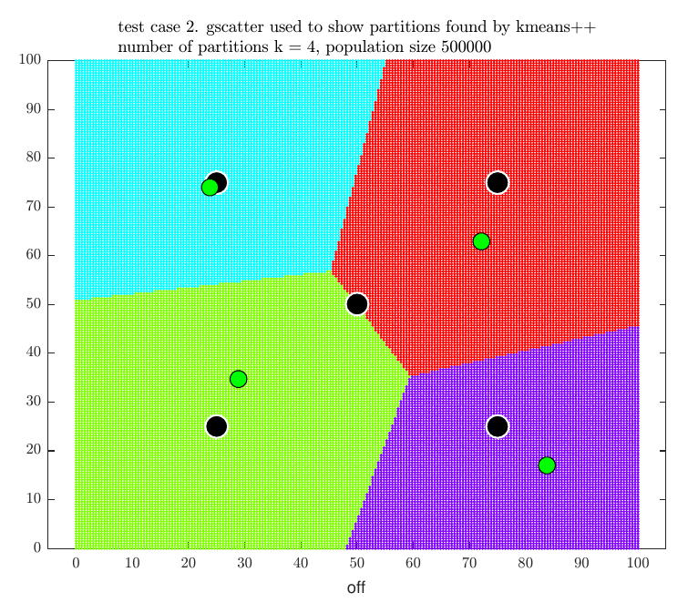
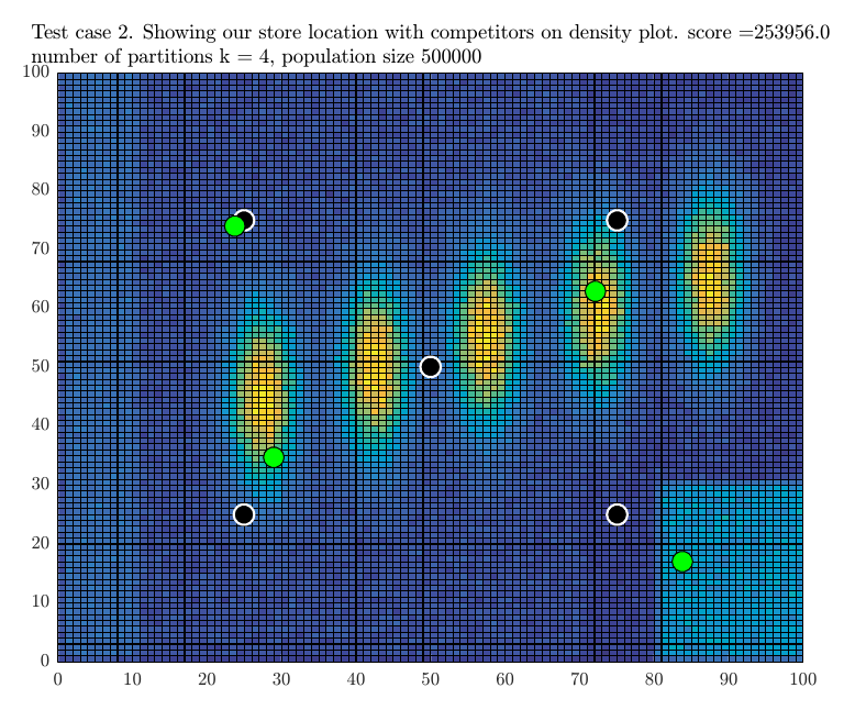
Before describing the algorithm below, we show an example using the early test send to us to illustrate how this method works. This used \(500,000\) population with \(5\) competitor stores (the black dots) in the plots that follows and \(n=4\) (the green dots).
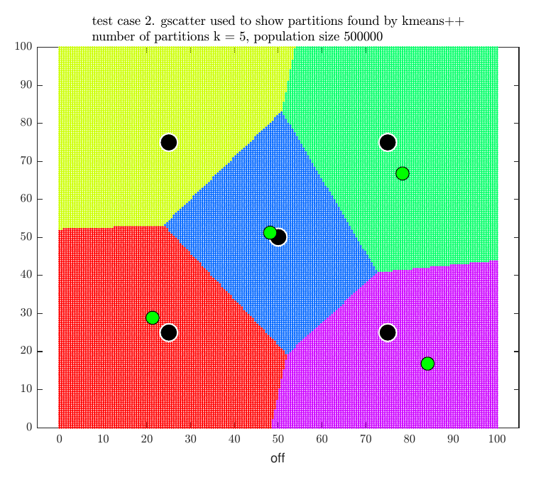
The partitions were now increased to \(5\) and \(5 \choose 4\) different combinations were scored to find the \(4\) best store locations out of these. This resulted in the following result
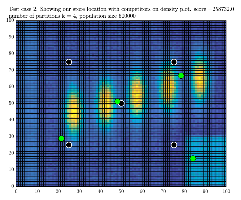
When trying \(6\) partitions, the score was decreased, so the search stopped. The program then printed the final result
This is a description of the algorithm which uses the kmeans++ cluster analysis function kmeans() as part of the Matlab Statistics and Machine Learning Toolbox toolbox, which is included in the student version. This is not a description of the kmeans++ algorithm itself, since that is well described and documented in many places such as in references [3,4]. This is a description of the algorithm using kmeans to solve the grocery location problem.

It was very important to check the correctness of the algorithm using small number of test cases to verify it is generating the optimal store locations as it is very hard to determine the optimal solution for any large size problem by hand. The following are some of the test problems used and the result obtained by the implementation, which shows that the optimal locations were found for each case.

By direct observations, since we have one store only, then we see that by locating it in the center of the population, the score will be \(6\), which is optimal. The optimal store location found by the program is \(\{2.333,2.222\}\)

Clearly when the competitor store is away from the density area, our score will increase. Since the competition also wants to increase its score, then it should also have to locate its store in the same location, which is the kmeans++ optimal location.

Many other test cases where run, using more store locations and they were verified manually that the program result agrees with the finding. It is not possible to verify manually that the result will remain optimal for large population and large number of stores, but these tests cases at least shows that the algorithm works as expected. Now we will show result of large tests cases and the program output generated.
The following table summarizes the result of running the store location algorithm on the 5 test cases provided.
| test case | n | m | X (population) | CPU time (minutes) | \(J^{\ast }\) | percentage |
| trial/earlier one | \(4\) | \(5\) | \(500,000\) | \(1.42\) | \(258,732\) | \(51.75\% \) |
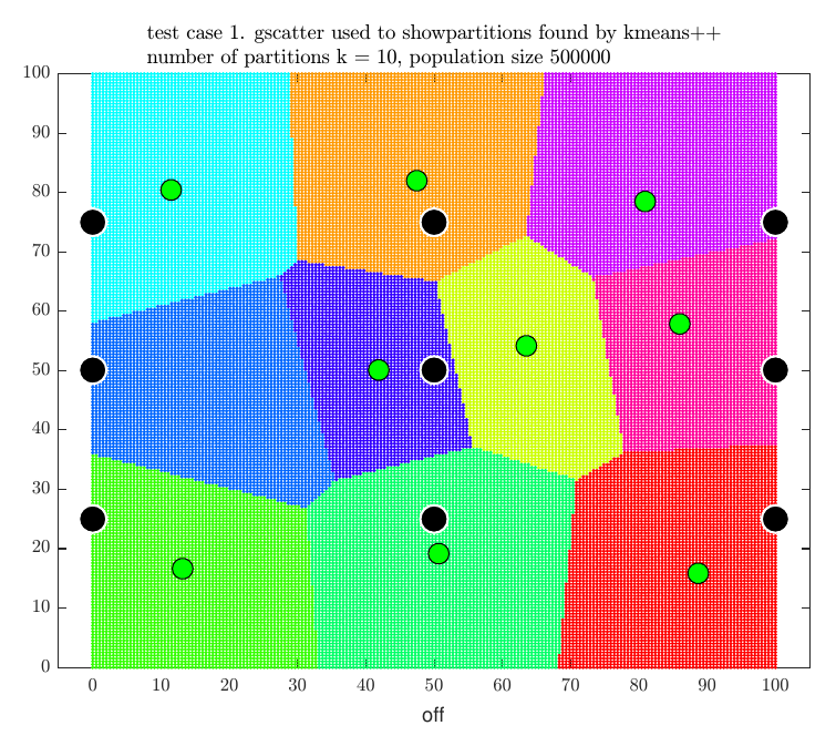
| \(1\) | \(9\) | \(9\) | \(500,000\) | \(5.49\) | \(371,543\) | \(74.32\% \) |
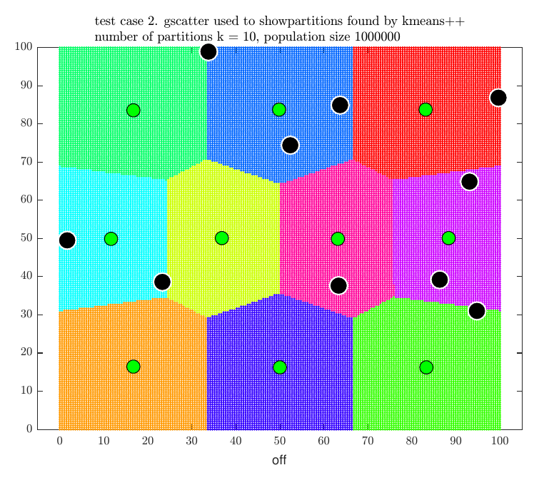
| \(2\) | \(10\) | \(10\) | \(1,000,000\) | \(3.38\) | \(637,413\) | \(63.74\% \) |
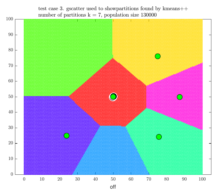
| \(3\) | \(5\) | \(5\) | \(130,000\) | \(1.16\) | \(69,093\) | \(53.15\% \) |
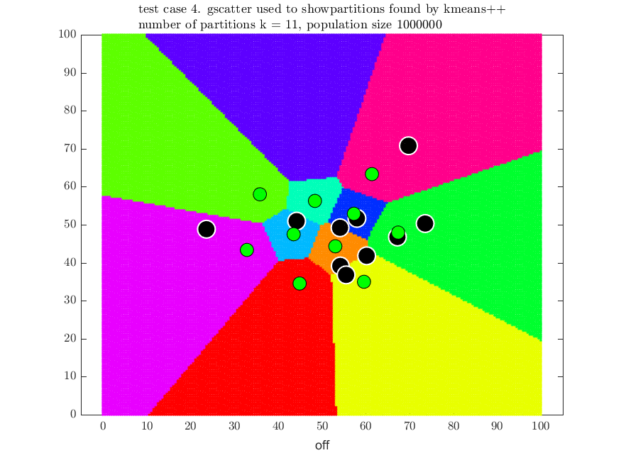
| \(4\) | \(10\) | \(10\) | \(1,000,000\) | \(14.17\) | \(683,899\) | \(68.39\% \) |
For illustration, the following four plots show the locations of our stores (the green dots) for the above final four test cases with the location of the competitor stores (black dots) and the final partitions selected.
kmeans++ algorithm for cluster analysis appears to be an effective method to use for finding an optimal store locations, but it is only practical for small \(n\) as the algorithm used to obtain the partitions is NP-hard. In addition \(p \choose n\) combinations of partitions needs to be searched to select the optimal set.
This implementation shows how kmeans++ can be used to solve these types of problems. The location of the competitor stores has no influence on where to locate the stores, but it only affects the final possible score. Generating more partitions (using kmeans++) than the number of stores and selecting from them the best set can lead to improved score. It was found in the test cases used that no more than two of three additional partitions than the number of stores was needed to find the a combination of partitions which gave the maximum score. Generating additional partitions made the score go lower. The score used is the number of customers the stores attract out of the overall population. The algorithm was verified to be correct for small number of tests cases (not shown here due to space limitation). More research is needed to investigate how feasible this method can be for solving similar resource allocations problems.