
Equation 7.7,11 b is\begin{equation} \frac{\Delta \theta \left ( s\right ) }{\delta _{e}\left ( s\right ) }=G_{\theta \delta _{e}}=\frac{b_{1}s+b_{0}}{sf\left ( s\right ) } \tag{7.7,11 b} \end{equation} Where \(f\left ( s\right ) =s^{2}+c_{1}s+c_{0}\). Using the hint, from (7.3,10), page 211 in the textbook\begin{align} f\left ( s\right ) & =s^{2}+c_{1}s+c_{0}\nonumber \\ & =s^{2}+2\zeta \omega _{n}s+\omega _{n}^{2}\nonumber \\ & =\left ( s-n\right ) ^{2}+\omega ^{2} \tag{7.3,10} \end{align}
Where \(n=-\zeta \omega _{n}\) and \(\omega =\omega _{n}\sqrt{\left ( 1-\zeta ^{2}\right ) }\,\). Substituting (7.3,10) into (7.7,11 b) gives\[ \frac{\Delta \theta \left ( s\right ) }{\delta _{e}\left ( s\right ) }=\frac{b_{1}s+b_{0}}{s\left ( \left ( s-n\right ) ^{2}+\omega ^{2}\right ) }\] Since \(\delta _{e}\left ( t\right ) \) is approximated as an impulse, its Laplace transform \(\delta _{e}\left ( s\right )\) is one. The above becomes\begin{equation} \Delta \theta \left ( s\right ) =\frac{b_{1}s+b_{0}}{s\left ( \left ( s-n\right ) ^{2}+\omega ^{2}\right ) }=\frac{b_{1}s+b_{0}}{s\left ( \underbrace{s^{2}-2ns+\left ( n^{2}+\omega ^{2}\right ) }_{\text{polynomial in s}} \right ) } \tag{1} \end{equation} To find \(\Delta \theta \left ( t\right )\), the inverse Laplace of the RHS of (1) is found using partial fractions. The polynomial in the denominator of (1) is in the following form\[ \frac{1}{x\left ( x^{2}+bx+c\right ) }\] From tables, the above has this partial fraction \[ \frac{A}{x}+\frac{Bx}{x^{2}+bx+c}+\frac{C}{x^{2}+bx+c}\] Therefore (1) can be written as \begin{align} \frac{b_{1}s+b_{0}}{s\left ( \left ( s-n\right ) ^{2}+\omega ^{2}\right ) } & =\frac{A}{s}+\frac{Bs}{s^{2}-2ns+\left ( n^{2}+\omega ^{2}\right ) }+\frac{C}{s^{2}-2ns+\left ( n^{2}+\omega ^{2}\right ) }\nonumber \\ & =\frac{A}{s}+\frac{Bs+C}{s^{2}-2ns+\left ( n^{2}+\omega ^{2}\right ) }\nonumber \\ & =\frac{A}{s}+\frac{Bs+C}{\left ( s-n\right ) ^{2}+\omega ^{2}} \tag{2} \end{align}
Expanding both sides and comparing powers of \(s\) of the numerators gives \begin{align*} b_{1}s+b_{0} & =A\left ( \left ( s-n\right ) ^{2}+\omega ^{2}\right ) +s\left ( Bs+C\right ) \\ & =A\left ( \left ( s^{2}+n^{2}-2ns\right ) +\omega ^{2}\right ) +Bs^{2}+Cs\\ & =As^{2}-2Ans+A\left ( n^{2}+\omega ^{2}\right ) +Bs^{2}+Cs\\ & =s^{2}\left ( A+B\right ) +s\left ( -2An+C\right ) +A\left ( n^{2}+\omega ^{2}\right ) \end{align*}
Comparing powers of \(s\) results in \begin{align*} b_{0} & =A\left ( n^{2}+\omega ^{2}\right ) \\ b_{1} & =-2An+C\\ 0 & =A+B \end{align*}
From the first equation above, \(A=\frac{b_{0}}{n^{2}+\omega ^{2}}\) and from the third equation \(B=-A=-\frac{b_{0}}{n^{2}+\omega ^{2}}\).
Using these, the second equation gives \begin{align*} C & =b_{1}+2An\\ & =b_{1}+\frac{2b_{0}n}{n^{2}+\omega ^{2}}\\ & =\frac{b_{1}\left ( n^{2}+\omega ^{2}\right ) +2b_{0}n}{n^{2}+\omega ^{2}} \end{align*}
Substituting the above values found for \(A,B,C\) into (2) results in \begin{align*} \Delta \theta \left ( s\right ) & =\frac{A}{s}+\frac{Bs+C}{\left ( s-n\right ) ^{2}+\omega ^{2}}\\ & =\frac{b_{0}}{n^{2}+\omega ^{2}}\frac{1}{s}+\frac{\frac{-b_{0}}{n^{2}+\omega ^{2}}s+\frac{b_{1}\left ( n^{2}+\omega ^{2}\right ) +2b_{0}n}{n^{2}+\omega ^{2}}}{\left ( s-n\right ) ^{2}+\omega ^{2}}\\ & =\frac{b_{0}}{n^{2}+\omega ^{2}}\frac{1}{s}+\frac{1}{n^{2}+\omega ^{2}}\frac{-b_{0}s+b_{1}\left ( n^{2}+\omega ^{2}\right ) +2b_{0}n}{\left ( s-n\right ) ^{2}+\omega ^{2}}\\ & =\left ( \frac{b_{0}}{n^{2}+\omega ^{2}}\right ) \frac{1}{s}-\frac{b_{0}}{\left ( n^{2}+\omega ^{2}\right ) }\left ( \frac{s-\frac{b_{1}}{b_{0}}\left ( n^{2}+\omega ^{2}\right ) -2n}{\left ( s-n\right ) ^{2}+\omega ^{2}}\right ) \end{align*}
Using Laplace transform tables5 the expression \(\frac{s-\alpha }{\left ( s-\alpha \right ) ^{2}+\omega ^{2}}\) is seen as closest to the above. To use the above expression, the second term above is converted to match it. Rewriting \(\Delta \theta (s)\) as \[ \Delta \theta \left ( s\right ) =\left ( \frac{b_{0}}{n^{2}+\omega ^{2}}\right ) \frac{1}{s}-\frac{b_{0}}{\left ( n^{2}+\omega ^{2}\right ) }\left ( \frac{\left ( s-n\right ) -\frac{b_{1}}{b_{0}}\left ( n^{2}+\omega ^{2}\right ) -n}{\left ( s-n\right ) ^{2}+\omega ^{2}}\right ) \] And breaking the second term on the RHS \begin{align} \Delta \theta \left ( s\right ) & =\left ( \frac{b_{0}}{n^{2}+\omega ^{2}}\right ) \frac{1}{s}-\frac{b_{0}}{\left ( n^{2}+\omega ^{2}\right ) }\left [ \frac{\left ( s-n\right ) }{\left ( s-n\right ) ^{2}+\omega ^{2}}-\frac{\frac{b_{1}}{b_{0}}\left ( n^{2}+\omega ^{2}\right ) +n}{\left ( s-n\right ) ^{2}+\omega ^{2}}\right ] \nonumber \\ & =\left ( \frac{b_{0}}{n^{2}+\omega ^{2}}\right ) \frac{1}{s}-\frac{b_{0}}{\left ( n^{2}+\omega ^{2}\right ) }\left [ \frac{\left ( s-n\right ) }{\left ( s-n\right ) ^{2}+\omega ^{2}}-\frac{1}{\omega }\left ( \frac{b_{1}}{b_{0}}\left ( n^{2}+\omega ^{2}\right ) +n\right ) \frac{\omega }{\left ( s-n\right ) ^{2}+\omega ^{2}}\right ] \tag{3} \end{align}
Using \(\frac{s-\alpha }{\left ( s-\alpha \right ) ^{2}+\omega ^{2}}\Rightarrow u\left ( t\right ) e^{\alpha t}\cos \left ( \omega t\right ) \) for the first part of the second term, and using \(\frac{\omega }{\left ( s-\alpha \right ) ^{2}+\omega ^{2}}\Rightarrow u\left ( t\right ) e^{\alpha t}\sin \omega t\) for the second part of the second term above, and since \(\frac{1}{s}\Rightarrow u\left ( t\right ) \) where \(u\left ( t\right ) \) in the above is the unit step function which can be factored out of all the terms since it is a common term. Now the inverse Laplace of (3) can be written as \[ \Delta \theta \left ( t\right ) =\left ( \frac{b_{0}}{n^{2}+\omega ^{2}}\right ) u\left ( t\right ) -\frac{b_{0}}{\left ( n^{2}+\omega ^{2}\right ) }\left [ e^{nt}\cos \left ( \omega t\right ) -\frac{1}{\omega }\left ( \frac{b_{1}}{b_{0}}\left ( n^{2}+\omega ^{2}\right ) +n\right ) e^{nt}\sin \left ( \omega t\right ) \right ] u\left ( t\right ) \] Therefore the time domain is\begin{equation} \boxed{ \Delta \theta \left ( t\right ) =\frac{b_{0}}{n^{2}+\omega ^{2}}-\frac{e^{nt}b_{0}\cos \left ( \omega t\right ) }{\left ( n^{2}+\omega ^{2}\right ) }+\frac{1}{\omega }\frac{b_{1}\left ( n^{2}+\omega ^{2}\right ) +n}{\left ( n^{2}+\omega ^{2}\right ) }e^{nt}\sin \left ( \omega t\right )} \tag{4} \end{equation} For \(t\geq 0\)
\(c_{1},c_{0}\) are now found in terms of \(n,\omega \). This is by definition from \begin{align} f\left ( s\right ) & =s^{2}+c_{1}s+c_{0}\nonumber \\ & =\left ( s-n\right ) ^{2}+\omega ^{2}\nonumber \\ & =s^{2}-2ns+\left ( \omega ^{2}+n^{2}\right ) \tag{7.3,10} \end{align}
Comparing terms gives \begin{align*} c_{1} & =-2n\\ c_{0} & =\omega ^{2}+n^{2} \end{align*}
Since \(n,\omega \) are known experimentally, using the above relation gives \(c_{1},c_{0}\).
To find \(b_{0}\) and \(b_{1}\), equation (4) in part (a) above is used, which is the solution as a function of time. \(n\) and \(\omega \) are known, therefore equation (4) has two unknowns: \(b_{1},b_{0}\). This requires two equations to solve. From the data, using \(\theta \left ( t_{1}\right ) \) and \(t_{1}\) generates one instance of equation (4) which is the solution at the instance \(t_{1}\). Another data set \(\theta \left ( t_{2}\right ) \) and \(t_{2}\) generates a second instance of the solution at \(t_{2}\).\begin{align*} \Delta \theta _{1}\left ( t_{1}\right ) & =\frac{b_{0}}{n^{2}+\omega ^{2}}-\frac{e^{nt_{1}}b_{0}\cos \left ( \omega t_{1}\right ) }{\left ( n^{2}+\omega ^{2}\right ) }+\frac{1}{\omega }\frac{b_{1}\left ( n^{2}+\omega ^{2}\right ) +n}{\left ( n^{2}+\omega ^{2}\right ) }e^{nt_{1}}\sin \left ( \omega t_{1}\right ) \\ \Delta \theta _{2}\left ( t_{2}\right ) & =\frac{b_{0}}{n^{2}+\omega ^{2}}-\frac{e^{nt_{2}}b_{0}\cos \left ( \omega t_{2}\right ) }{\left ( n^{2}+\omega ^{2}\right ) }+\frac{1}{\omega }\frac{b_{1}\left ( n^{2}+\omega ^{2}\right ) +n}{\left ( n^{2}+\omega ^{2}\right ) }e^{nt_{2}}\sin \left ( \omega t_{2}\right ) \end{align*}
These two equations can be solved numerically simultaneously for \(b_{0},b_{1}\). All the parameters in (4) are now known: \(\left \{ b_{0},b_{1},n,\omega \right \}\). The solution as given in (4) is now found and can be simulated or plotted as needed.

solution
The eight transfer functions are given in equation (7.9,5)\begin{align*} G_{v,\delta _{a}}\left ( s\right ) & =\frac{N_{v,\delta a}\left ( s\right ) }{f\left ( s\right ) }=\frac{2.896s^{2}+6.542s+0.622}{f\left ( s\right ) }\\ G_{v,\delta r}\left ( s\right ) & =\frac{N_{v,\delta r}\left ( s\right ) }{f\left ( s\right ) }=\frac{5.642s^{3}+379.4s^{2}+167.9s-5.934}{f\left ( s\right ) }\\ G_{p,\delta _{a}}\left ( s\right ) & =\frac{N_{p,\delta a}\left ( s\right ) }{f\left ( s\right ) }=\frac{0.1431s^{3}+0.0273s^{2}+0.1102s}{f\left ( s\right ) }\\ G_{p,\delta r}\left ( s\right ) & =\frac{N_{p,\delta r}\left ( s\right ) }{f\left ( s\right ) }=\frac{0.1144s^{3}-0.1997s^{2}-1.368s}{f\left ( s\right ) }\\ G_{r,\delta _{a}}\left ( s\right ) & =\frac{N_{r,\delta a}\left ( s\right ) }{f\left ( s\right ) }=\frac{-0.003741s^{3}-0.002708s^{2}-0.0001394s+0.004539}{f\left ( s\right ) }\\ G_{r,\delta r}\left ( s\right ) & =\frac{N_{r,\delta r}\left ( s\right ) }{f\left ( s\right ) }=\frac{-0.4849s^{3}-0.2327s^{2}-0.009018s-0.05647}{f\left ( s\right ) }\\ G_{\phi ,\delta _{a}}\left ( s\right ) & =\frac{N_{\phi ,\delta a}\left ( s\right ) }{f\left ( s\right ) }=\frac{0.1431s^{2}+0.0273s+0.1102}{f\left ( s\right ) }\\ G_{\phi ,\delta r}\left ( s\right ) & =\frac{N_{\phi v,\delta r}\left ( s\right ) }{f\left ( s\right ) }=\frac{0.1144s^{2}-0.1997s-1.368}{f\left ( s\right ) } \end{align*}
Where \begin{equation} \boxed{ f\left ( s\right ) =s^{4}+0.6358s^{3}+0.9388s^{2}+0.5114s+0.003682} \tag{6.7,2} \end{equation}
To find the static gain, equation (7.4,5) is used, which says\begin{equation} k=\lim _{s\rightarrow 0}G_{ij}\left ( s\right ) \tag{7.5,4} \end{equation} The above is applied to each of the transfer functions in (7.9,5)\begin{align*} K_{v,\delta _{a}} & =\lim _{s\rightarrow 0}G_{v,\delta _{a}}\left ( s\right ) =\lim _{s\rightarrow 0}\frac{2.896s^{2}+6.542s+0.622}{s^{4}+0.6358s^{3}+0.9388s^{2}+0.5114s+0.003682}=\frac{0.622}{0.003682}=168.\,\allowbreak 93\\ K_{v,\delta r} & =\lim _{s\rightarrow 0}G_{v,\delta r}\left ( s\right ) =\lim _{s\rightarrow 0}\frac{5.642s^{3}+379.4s^{2}+167.9s-5.934}{s^{4}+0.6358s^{3}+0.9388s^{2}+0.5114s+0.003682}=\frac{-5.934}{0.003682}=-1611.\,\allowbreak 6\\ K_{p,\delta _{a}} & =\lim _{s\rightarrow 0}G_{p,\delta _{a}}\left ( s\right ) =\lim _{s\rightarrow 0}\frac{0.1431s^{3}+0.0273s^{2}+0.1102s}{s^{4}+0.6358s^{3}+0.9388s^{2}+0.5114s+0.003682}=0\\ K_{p,\delta r} & =\lim _{s\rightarrow 0}G_{p,\delta r}\left ( s\right ) =\lim _{s\rightarrow 0}\frac{0.1144s^{3}-0.1997s^{2}-1.368s}{s^{4}+0.6358s^{3}+0.9388s^{2}+0.5114s+0.003682}=0\\ K_{r,\delta _{a}} & =\lim _{s\rightarrow 0}G_{r,\delta _{a}}\left ( s\right ) =\lim _{s\rightarrow 0}\frac{-0.003741s^{3}-0.002708s^{2}-0.0001394s+0.004539}{s^{4}+0.6358s^{3}+0.9388s^{2}+0.5114s+0.003682}=\frac{0.004539}{0.003682}=1.\,\allowbreak 232\,8\\ K_{r,\delta r} & =\lim _{s\rightarrow 0}G_{r,\delta r}\left ( s\right ) =\lim _{s\rightarrow 0}\frac{-0.4849s^{3}-0.2327s^{2}-0.009018s-0.05647}{s^{4}+0.6358s^{3}+0.9388s^{2}+0.5114s+0.003682}=\frac{-0.05647}{0.003682}=-15.\,\allowbreak 337\\ K_{\phi ,\delta _{a}} & =\lim _{s\rightarrow 0}G_{\phi ,\delta _{a}}\left ( s\right ) =\lim _{s\rightarrow 0}\frac{0.1431s^{2}+0.0273s+0.1102}{s^{4}+0.6358s^{3}+0.9388s^{2}+0.5114s+0.003682}=\frac{0.1102}{0.003682}=29.\,\allowbreak 929\\ K_{\phi ,\delta r} & =\lim _{s\rightarrow 0}G_{\phi ,\delta r}\left ( s\right ) =\lim _{s\rightarrow 0}\frac{0.1144s^{2}-0.1997s-1.368}{s^{4}+0.6358s^{3}+0.9388s^{2}+0.5114s+0.003682}=\frac{-1.368}{0.003682}=-371.\,\allowbreak 54 \end{align*}
The slope for large frequency is determined for all the above transfer functions using the following method. The first step is to write the transfer function in a polynomial factored form (in Matlab, called zpk form). This results in the following form of the transfer function\[ G\left ( s\right ) =\frac{k\left ( s+z_{1}\right ) \left ( s+z_{2}\right ) \cdots \left ( s+z_{n}\right ) }{s\left ( s+p_{1}\right ) \left ( s+p_{2}\right ) \cdots \left ( s+p_{m}\right ) }\] Where the \(z_{i}\) are the zeros of the numerator polynomial, and the \(p_{i}\) are the poles of the denominator polynomial.
\(s\) is now replaced by \(j\omega \) and each factored term is converted to \(\left ( 1+j\frac{\omega }{z_{i}}\right ) \) in the numerator and to \(\left ( 1+j\frac{\omega }{p_{i}}\right ) \) in the denominator. This requires factoring out a \(z_{i}\) or \(p_{i}\). This converts \(G\left ( s\right )\) to a standard form for corner frequency analysis in the bode plot.\begin{align*} G\left ( s\right ) & =\frac{k\frac{z_{1}z_{2}\cdots z_{n}}{p_{1}p_{2}\cdots p_{m}}\left ( 1+j\frac{\omega }{z_{1}}\right ) \left ( 1+j\frac{\omega }{z_{2}}\right ) \cdots \left ( 1+j\frac{\omega }{z_{n}}\right ) }{s\left ( 1+j\frac{\omega }{p_{1}}\right ) \left ( 1+j\frac{\omega }{p_{2}}\right ) \cdots \left ( 1+j\frac{\omega }{p_{n}}\right ) }\\ & =\left ( k\frac{z_{1}z_{2}\cdots z_{n}}{p_{1}p_{2}\cdots p_{m}}\right ) \frac{\left ( 1+j\frac{\omega }{z_{1}}\right ) \left ( 1+j\frac{\omega }{z_{2}}\right ) \cdots \left ( 1+j\frac{\omega }{z_{n}}\right ) }{\left ( j\omega \right ) \left ( 1+j\frac{\omega }{p_{1}}\right ) \left ( 1+j\frac{\omega }{p_{2}}\right ) \cdots \left ( 1+j\frac{\omega }{p_{n}}\right ) } \end{align*}
In the above, \(z_{i}\) and \(p_{i}\) are corner frequencies. At a corner frequency the slope changes by \(+20\) db/decade at each zero \(z_{i}\), and changes by \(-20\) db/decade for the each pole \(p_{i}\).
Therefore when a corner frequency in the numerator is reached, the slope of the bode log magnitude increases by additional \(20\) db/decade and when a corner frequency \(p_{i}\) in the denominator is reached, the slope of the bode log magnitude decreases by \(20\) db/decade. The slope starts at \(-20\) db/decade due to the \(\left ( j\omega \right ) \) term in the denominator. This term has no corner frequency but it has slope of \(-20\) db/decade.
Using this form of the transfer function, to find the slope for large frequency, \(20\) db/decade is added for each zero and \(20\) db/decade is subtracted for each pole. This is done for all corner frequencies until all frequencies are counted for. The final slope that results, is the slope needed, which is the slope at large frequency.
Since the number of zeros is the same as the degree of the numerator polynomial, and the number of poles is the same as the degree of the denominator polynomial, the difference between the degrees gives the final slope in db per decade. In this problem the number of poles is \(4\) for all the transfer functions since that is the common polynomial \(f\left ( s\right ) \).
The final slope is converted to decade per decade since \(20\) db per decade is one decade per decade. The table below summarizes the result
| Transfer function | zeros | poles | large frequency slope | slope (decade/decade) |
| \(G_{v,\delta _{a}}\left ( s\right ) \) | \(2\) | \(4\) | \(\left ( 2-4\right ) =-2\Rightarrow -40\) db/dec | \(-2\) |
| \(G_{v,\delta r}\left ( s\right ) \) | \(3\) | \(4\) | \(\left ( 3-4\right ) =-1\Rightarrow -20\) db/dec | \(-1\) |
| \(G_{p,\delta _{a}}\left ( s\right ) \) | \(3\) | \(4\) | \(\left ( 3-4\right ) =-1\Rightarrow -20\) db/dec | \(-1\) |
| \(G_{p,\delta r}\left ( s\right ) \) | \(3\) | \(4\) | \(\left ( 3-4\right ) =-1\Rightarrow -20\) db/dec | \(-1\) |
| \(G_{r,\delta _{a}}\left ( s\right ) \) | \(3\) | \(4\) | \(\left ( 3-4\right ) =-1\Rightarrow -20\) db/dec | \(-1\) |
| \(G_{r,\delta r}\left ( s\right ) \) | \(3\) | \(4\) | \(\left ( 3-4\right ) =-1\Rightarrow -20\) db/dec | \(-1\) |
| \(G_{\phi ,\delta _{a}}\left ( s\right ) \) | \(2\) | \(4\) | \(\left ( 2-4\right ) =-2\Rightarrow -40\) db/dec | \(-2\) |
| \(G_{\phi ,\delta r}\left ( s\right ) \) | \(2\) | \(4\) | \(\left ( 2-4\right ) =-2\Rightarrow -40\) db/dec | \(-2\) |
To make it easier to answer this question, block diagrams are used for the transfer functions. The following diagram shows the 8 transfer functions in (7.9,5) in block diagrams. The input is the control signal, and the output is the result of multiplying the control signal by the transfer function.

To find the output from the transfer function, the input to the transfer function is multiplied by the transfer function itself. For example, looking at the last transfer function block diagram in the aileron transfer functions above, the following determines \(\phi \) \[ \phi =\delta _{a}G_{\phi \delta _{a}}\]
The above from the definition of the transfer function, since \(G_{\phi \delta _{a}}=\frac{output}{input}=\frac{\phi }{\delta _{a}}\). The input to the transfer function block is the control signal.
The problem says that \(\omega =\SI{0}{\radian \per \second }\), which is the steady state. But \(k=\lim _{s\rightarrow 0}G_{ij}\left ( s\right ) \) from part (a). This means the transfer function in the above block diagram becomes the static gain. Each \(G\left ( s\right ) \) is replaced by the corresponding gain found in part (a).

Aileron controls For the aileron control \[ \phi =\delta _{a}G_{\phi \delta _{a}}\] using \(\phi =15^{0}=15\left ( \frac{\pi }{180}\right ) =\SI{0.26180}{\radian }\) the above becomes \begin{align*} 0.261\,80 & =\delta _{a}\times 29.929\\ \delta _{a} & =\frac{0.26180}{29.929}\\ & =8.7474\times 10^{-3}\text{ radian}\\ & =8.7474\times 10^{-3}\left ( \frac{180}{\pi }\right ) \\ & =\boxed{\SI{0.50119}{\degree }} \end{align*}
This is the aileron control angle that produces \(\phi =15^{o}\) in steady state. The problem now asks to find \(\beta \), the side slip angle. The side slip angle is

And given in equation (1.6,4) in the textbook as \begin{equation} \beta =\tan ^{-1}\left ( \frac{v}{V}\right ) \tag{1.6,4} \end{equation} Where \(v\) is the speed in the lateral direction and \(V\) is the magnitude of the velocity vector of the airplane. The example used in this problem is based on the same jet section 6.2, page 165 of the textbook, shown in the figure below.
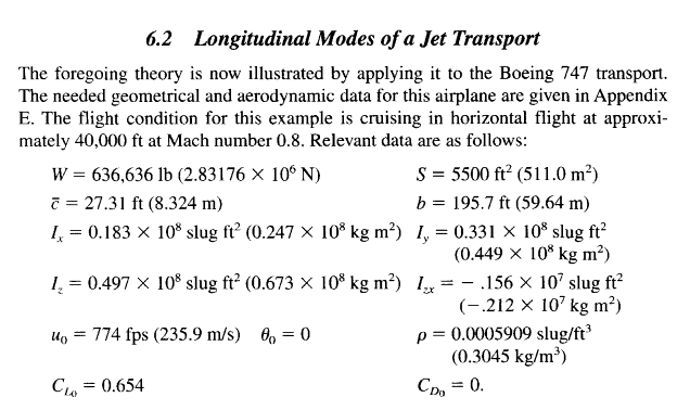
From the above \(u_{o}=\SI{774}{\ft \per \second }\). Using this in (1.6,4) gives \begin{equation} \beta =\tan ^{-1}\left ( \frac{v}{774}\right ) \tag{2} \end{equation} \(v\) is now found in order to find \(\beta \). From the above transfer functions, using the first one gives \(v\)

Therefore \(v=\delta _{a}\left ( 168.93\right ) \) but \(\delta _{a}=\SI{0.50119}{\degree }\) from above. Hence\begin{align*} v & =\left ( 0.50119^{o}\times \frac{\pi }{180}\right ) \left ( 168.93\right ) \\ & =\SI{1.4777}{\ft \per \second } \end{align*}
Substituting \(v\) from above in (2) gives\begin{align*} \beta & =\tan ^{-1}\left ( \frac{v}{774}\right ) \\ & =\tan ^{-1}\left ( \frac{1.4777}{774}\right ) \\ & =\SI{0.0019}{\radian }\\ & =\SI{0.1094}{\degree } \end{align*}
To find the yaw rate \(r\), the following transfer function is used

Hence \begin{align*} r & =\delta _{a}\left ( 1.2328\right ) \\ & =\left ( 0.50119^{o}\times \frac{\pi }{180}\right ) \left ( 1.2328\right ) \\ & =\SI{0.010784}{\radian \per \second }\\ & =\boxed{\SI{0.61788}{\degree \per \second }} \end{align*}
The same process is repeated using the the rudder control blocks on the right side of the above figure. These are the blocks that takes \(\delta _{r}\) as control signal.
For the rudder control \[ \phi =\delta _{r}G_{\phi \delta _{r}}\] For \(\phi =15^{0}=15\left ( \frac{\pi }{180}\right ) =\SI{0.2618}{\radian }\), the above becomes \begin{align*} 0.2618 & =\delta _{r}\times \left ( -371.54\right ) \\ \delta _{r} & =\frac{0.2618}{-371.54}\\ & =-7.046\,3\times 10^{-4}\text{ radian}\\ & =-0.0404^{o} \end{align*}
This is the rudder control angle that produces \(\phi =\SI{15}{\degree }\) in steady state. The problem now asks to find \(\beta \), the side slip angle. Using \begin{equation} \beta =\tan ^{-1}\left ( \frac{v}{744}\right ) \tag{2} \end{equation} \(v\) is now found in order to find \(\beta \). From the above blocks, using the block that output \(v\) from a rudder control signal gives

Therefore \(v=\delta _{r}\left ( -1611.6\right ) \). But \(\delta _{r}=\SI{-0.0404}{\degree }\) from above. Hence\begin{align*} v & =\left ( -0.0404^{o}\times \frac{\pi }{180}\right ) \left ( -1611.6\right )\\ & =\SI{1.1364}{\ft \per \second } \end{align*}
Substituting this \(v\) in (2) gives\begin{align*} \beta & =\tan ^{-1}\left ( \frac{v}{744}\right ) \\ & =\tan ^{-1}\left ( \frac{1.1364}{744}\right ) \\ & =\SI{0.0015}{\radian }\\ & =\boxed{\SI{0.0841}{\degree }} \end{align*}
To find the yaw rate \(r\), the following block which output \(r\) for input \(\delta _{r}\) is used

Hence \begin{align*} r & =\delta _{r}\left ( -15.337\right ) \\ & =\left ( \SI{-0.0404}{\degree }\times \frac{\pi }{180}\right ) \left ( -15.337\right ) \\ & =\SI{0.010814}{\radian \per \second }\\ & =\boxed{\SI{0.6196}{\degree \per \second }} \end{align*}

solution:
The load factor \(n_{z}\) is the ratio of lift to weight \begin{equation} n_{z}=\frac{L}{W}=\frac{-Z}{W} \tag{7.7,4} \end{equation}
\(n_{z}\) is unity for straight horizontal steady flight6 . The minus sign on the \(Z\) force is added since \(Z\) is positive downwards (in body coordinates of the airplane) while the lift \(L\) is upwards. The transfer function in figure 7.18 is defined as
\begin{equation} G_{\Delta n_{z},\delta _{e}}=\frac{\Delta n_{z}}{\delta _{e}} \tag{1} \end{equation} In block transfer function diagram the above is

Where7 \[ n_{z}=n_{z_{0}}+\Delta n_{z}\] \(n_{z_{0}}\) is the load factor \(n_{z}\) at trim defined as one. Hence the above becomes\begin{equation} \boxed{n_{z}=1+\Delta n_{z}} \tag{2} \end{equation} Figure 7.18 shows that \(\left \vert G_{\Delta n_{z},\delta _{e}}\right \vert =15\) when \(\omega \) is close to the short term frequency.
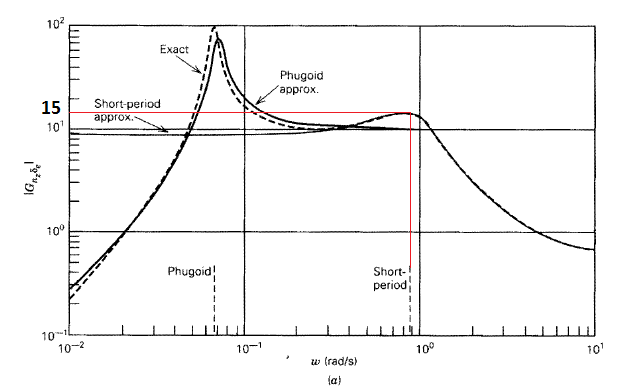
Therefore (1) becomes\begin{align*} 15 & =\frac{\Delta n_{z}}{2\times \frac{\pi }{180}}\\ \Delta n_{z} & =2\times \frac{\pi }{180}\times 15\\ & =0.52360 \end{align*}
Using (2), the load factor \(n_{z}\) is now found\begin{align*} n_{z} & =1+0.52360\\ & =\boxed{1.5236} \end{align*}
If a passenger at exactly the CG of the airplane floats up from the seat, it implies no external force \(Z\) acting down at the C.G. In other words, this is the same as saying the lift \(L\) is zero. So the airplane has only its weight \(W\) acting downwards (this is similar to having an airplane in free fall and moving with constant horizontal velocity as used to simulate being in outer space). When \(L=0\) then \(n_{z}=0\). From (2)
\begin{align*} 0 & =1+\Delta n_{z}\\ \Delta n_{z} & =-1 \end{align*}
And from (1)\begin{align*} G_{\Delta n_{z},\delta _{e}} & =\frac{\Delta n_{z}}{\delta _{e}}\\ 15 & =\frac{-1}{\delta _{e}}\\ \delta _{e} & =\frac{-1}{15}=\SI{-0.06667}{\radian } \end{align*}
Hence the elevator angle needed is
\[ \boxed{\delta _{e}= \SI{-3.82}{\degree }} \]
For \(n_{z}=2.5\)
\begin{align*} 2.5 & =1+\Delta n_{z}\\ \Delta n_{z} & =2.5-1\\ & =1.5 \end{align*}
Hence from (1)
\begin{align*} 15 & =\frac{1.5}{\delta _{e}}\\ \delta _{e} & =\frac{1.5}{15}\\ & =0.1\text{ radian} \end{align*}
Therefore
\[ \boxed{\delta _{e}=\SI{5.7296}{\degree }} \]

solution:
The summary of observations is given first. In longitudinal control, elevator action \(\delta _e\) and thrust action \(\delta _p\) can be applied separately from each others to achieve the expected response for each control. In lateral control, the rudder action \(\delta _r\) and the aileron action \(\delta _a\) have to be applied simultaneously to achieve the expected response for roll and yaw motion. For side slip rate (lateral speed \(v\)) rudder control \(\delta _r\) was the primary control needed.
Once the transfer functions are found, all the required plots are generated using Matlab. Each plot generated has the Matlab code used to generate above it. In addition to the response plots, Bode plots were generated to verify the output with the textbook.
Table 2.1 gives a summary of the variables to control for each mode of motion.
| type of motion | variable | meaning |
|
Longitudinal |
\(\Delta u\) | Velocity component in the \(x\) direction (cruise speed) |
| \(w\) | Velocity component in the \(z\) direction | |
| \(q\) | Pitch rate | |
| \(\Delta \theta \) | pitch angle | |
|
Lateral |
\(v\) | Side slip rate or side velocity. |
| \(p\) | Roll rate | |
| \(r\) | Yaw rate | |
| \(\Delta \phi \) | Bank angle | |
results and observations found for longitudinal motion Table 2.2 summarizes the results and observations found for longitudinal motion.
| Control action |
Numerator of planet transfer function |
Observed response and comments |
|
\(\delta _e=\SI{1}{\degree }\)
elevator
angle.
positive
is
down.
causes
changes
in
pitch
angle
\(\alpha \)
which
in
steady
state
is
meant
to
cause
change
in
cruise
speed
only |
\(N_{u,\delta _e}\) |
Increases cruise speed as expected, but too slowly. 10 minutes needed to reach steady state. All the response happens in phugoid mode. Large overshoot, with oscillations in response due to low damping in phugoid. Reference figure 7.19, figure 7.20 in textbook |
|
|
\(N_{\alpha ,\delta _e}\) |
Angle of attack responds fast, in short period mode, rapidly damped. 5 minutes to reach steady state with small residual seen present in steady state. Reference figure 7.19, figure 7.20 in textbook |
|
|
\(N_{\gamma ,\delta _e}\) |
Response contained in phugoid, slow (10 minutes) with remaining \(\gamma \) angle residual remaining. Which implies a residual \(\Delta _\alpha \) residual exists as a result. Something that was supposed to be generated. Reference figure 7.19, figure 7.20 in textbook |
|
\(\delta _p=\frac{1}{6}\)
Throttle
(thrust).
Causes
climb
up
or
down.
In
other
words,
this
control
action
is
used
to
cause
a
change
\(\Delta _\theta \).
No
change
in
\(\Delta u\)
nor
in
angle
of
attack
\(\alpha \)
should
result
if
thrust
lines
pass
through
C.G. |
\(N_{u,\delta _p}\) |
\(\Delta u\) Remained unchanged as expected but only after initial undesired oscillations. Took 20 minutes to damp out completely. |
|
|
\(N_{\alpha ,\delta _p}\) |
Remained unchanged as expected with very little oscillation. Damps out after 200 seconds. |
|
|
\(N_{\gamma ,\delta _e}\) |
2.8° steady state response reached after 10 minutes. Large overshoot. Many oscillations before damping out. |
|
\(\delta _p + \delta _e\)
Simultaneous
effect
of
applying
both
controls
at
same
time |
\(N_{u,(\delta _p+\delta _e)}\) |
Throttle action has almost no effect on speed \(\Delta u\) response, other than causing a small increase in overshoot and slight phase delay in oscillations compared to \(\delta _e\) only control. Slow response as before. |
|
|
\(N_{\alpha ,(\delta _p+\delta _e)}\) |
Throttle action \(\delta _p\) also had almost no effect on angle of attack response. Response followed very closely the \(\delta _e\) response as described above. |
|
|
\(N_{\gamma ,(\delta _p+\delta _e)}\) |
In this case, the addition of elevator action was seen to have most effect on transient response of flight path angle. Steady state remained as with throttle action alone, but adding elevator action caused large overshoot compared to throttle only response. Also a phase shift was seen. Steady state was slow to be reached as with throttle only action. |
results and observations found for lateral motion Table 2.3 summarizes the results and observations found for lateral motion when each control is applied separately.
| Control action |
Numerator of plant transfer function |
Observed response and comments |
|
\(\delta _r=\SI{3}{\degree }\)
Causes
Yaw
motion. |
\(N_{\nu ,\delta _r}\) |
Rudder affects initial side slip rate much more than aileron. After 10 minutes, \(\nu \) reached −80 ft s−1 at steady state. High oscillatory response and faster response compared to aileron \(\delta _a\) only. |
|
|
\(N_{p,\delta _r}\) |
2 minutes was needed to reach steady state of −0.04 rad s−1 , high overshoot, similar to aileron with oscillation. Aileron \(\delta _a\) caused similar effect. |
|
|
\(N_{r,\delta _r}\) |
Took 10 minutes to reach steady state of −0.8 rad s−1 compared to aileron \(\delta _a\) case, which needed 20 minutes to cause only −0.12 rad s−1 change. But small oscillation seen in the first minute of response. |
|
|
\(N_{\phi ,\delta _r}\) |
Much more effect on bank angle than aileron. In 6 minutes this action caused −19° change in bank angle. Smooth response. |
|
\(\delta _a=\SI{6}{\degree }\)
Causes
roll
motion | \(N_{\nu ,\delta _a}\) | After 10 minutes reached steady state of only −18 ft s−1 compared to −80 ft s−1 by rudder \(\delta _r\) in the same amount of time. Side slip rate is seen to be more controlled by rudder alone. |
|
|
\(N_{p,\delta _a}\) |
2 minutes to reach steady state of −0.006 rad s−1, high overshoot, similar to rudder with oscillation. But rudder 3° input caused much larger roll rate of −0.04 rad s−1 |
|
|
\(N_{r,\delta _a}\) |
Took 20 minutes to reach steady state of −0.12 rad s−1 , Smooth response, no oscillation. Rudder response was similar but rudder response reached steady state in half the time (10 minutes) and had much larger effect on yaw rate. |
|
|
\(N_{\phi ,\delta _a}\) |
Less affect on bank angle compared to rudder. After same amount of 10 minutes, cause only −3° change in bank angle compared to about −20° with the above rudder input. |
Table 2.4 summarizes the results and observations found for lateral motion when both controls \(\delta _p\) and \(\delta _r\) are applied simultaneously.
| Control action |
Numerator of plant transfer function |
Observed response and comments |
|
\(\delta _r+\delta _a\)
where
\(\delta _r=\SI{+3}{\degree }\)
and
\(\delta _a=\SI{+6}{\degree }\) |
\(N_{\nu ,(\delta _r+\delta _a)}\) |
Combined side slip rate response followed the rudder only response. Aileron control response had small effect on final speed. Steady state reached in 10 minutes to about −100 ft s−1 compared to −80 ft s−1 with rudder alone. |
|
|
\(N_{r,(\delta _r+\delta _a)}\) |
Yaw rate response is controlled mainly by Rudder. Aileron had little effect. Initial small oscillation was still present in combined response. Damped out after one minute. |
|
|
\(N_{\phi ,(\delta _r+\delta _a)}\) |
Combined response followed rudder response. Aileron effect on bank angle is minimal. |
|
\(\delta _r+\delta _a\)
where
\(\delta _r=\SI{-3}{\degree }\)
and
\(\delta _a=\SI{+6}{\degree }\) |
\(N_{\nu ,(\delta _r+\delta _a)}\) |
Combined side slip rate response followed the rudder only response. Aileron control response had small effect on final speed. Steady state was reached in 10 minutes to about 70 ft s−1 compared to 80 ft s−1 with rudder alone. Aileron effect has reduced final speed by 10 ft s−1 |
|
|
\(N_{r,(\delta _r+\delta _a)}\) |
Yaw rate response is controlled mainly by Rudder. Aileron had little effect. Initial small oscillation still present in combined response. Damped out after one minute. |
|
|
\(N_{\phi ,(\delta _r+\delta _a)}\) |
Combined response followed rudder response. Aileron effect on bank angle is minimal. |
To obtain the transfer function matrix \(G_{ij}\left ( s\right ) \) for the longitudinal motion, the following matrix is found
\begin{equation} \mathbf{G}\left ( s\right ) =\left ( s\mathbf{I}-\mathbf{A}\right ) ^{-1}\mathbf{B} \tag{1} \end{equation} Where \(A\) is the matrix for B-747 given on page 166, and \(B\) is given on page 229. The equation of motion for longitudinal motion becomes\[\begin{pmatrix} \Delta \dot{u}\\ \dot{w}\\ \dot{q}\\ \Delta \dot{\theta }\end{pmatrix} =\overset{A}{\overbrace{\begin{pmatrix} -0.006868 & 0.01395 & 0 & -32.2\\ -0.09055 & -0.3151 & 773.98 & 0\\ 0.000118 & -0.001026 & -0.4285 & 0\\ 0 & 0 & 1 & 0 \end{pmatrix} }}\overset{\text{output}}{\overbrace{\begin{pmatrix} \Delta u\\ w\\ q\\ \Delta \theta \end{pmatrix} }}+\overset{B}{\overbrace{\begin{pmatrix} -0.000187 & 9.66\\ -17.85 & 0\\ -1.158 & 0\\ 0 & 0 \end{pmatrix} }}\overbrace{\begin{Bmatrix} \delta _{e}\\ \delta _{p}\end{Bmatrix} }^{\text{control input}}\] Once \(G\left ( s\right ) \) is found, it will be a \(4\times 2\) matrix. \(G\left ( i,j\right ) \) is the transfer function of the ratio of \(i^{th}\) output to the \(j^{th}\) input. For example, \(G_{\Delta u,\delta _{e}}\) will be \(G\left ( 1,1\right ) \) which is a function of \(s\) in equation (1). To obtain all the transfer functions, equation (1) is evaluated. This can be done using equation 7.2.7 on page 209\begin{align*} \left ( s\mathbf{I}-\mathbf{A}\right ) ^{-1}&=\frac{adj\left ( s\mathbf{I}-\mathbf{A}\right ) }{\det \left ( s\mathbf{I}-\mathbf{A}\right ) } \end{align*}
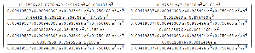
For this problem, finding the transfer functions is done using computer algebra. Here are the steps and the resulting \(G\left ( s\right ) \) matrix.
Which gives the following result
Using Matlab, the same procedure was also performed using symbolic toolbox as follows
The output generated is
Generating the transfer function when throttle \(\delta _{p}\) is the input \(G_{ij}\) is now found to solve the problem. The input is the throttle \(\delta _{p}\) which is \(j=2\). The output in figure 7.21 top plot is \(\Delta u\), which is \(i=1\). Therefore \begin{equation} G_{12}\left ( s\right ) =G_{\Delta u,\delta _{p}}=\frac{ \overbrace{-9.66s^{3}+7.18218s^{2}+8.97534s}^{N_{u,\delta _{p}}} }{s^{4}+0.750468s^{3}+0.935494s^{2}+0.00946303s+0.00419587} \tag{2} \end{equation}
To obtain the transfer function for the second plot, the transfer function for the angle of attack is needed. But \(\alpha =\frac{w}{u_{0}}\) where \(u_{0}=\SI{774}{\ft \per \second }\), which is the cruise speed. Therefore \(N_{\alpha ,\delta _{p}}=\frac{1}{u_{0}}N_{w,\delta _{p}}\). But what is \(N_{w,\delta _{p}}\) ?. Since \(\delta _{p}\) is the second input, then \(j=2\) and since \(w\) is the second output then \(i=2\), therefore \[ G_{w,\delta _{p}}=G_{2,2}=\frac{-0.874713s^{2}+0.512663s}{s^{4}+0.750468s^{3}+0.935494s^{2}+0.00946303s+0.00419587}\]
Hence\begin{align} G_{\alpha ,\delta _{p}} & =\frac{G_{2,2}}{u_{0}}\nonumber \\ & =\frac{1}{774}\frac{-0.874713s^{2}+0.512663s}{s^{4}+0.750468s^{3}+0.935494s^{2}+0.00946303s+0.00419587}\nonumber \\ & =\frac{0.0006624s-0.00113s^{2}}{s^{4}+0.750468s^{3}+0.935494s^{2}+0.00946303s+0.00419587} \tag{3} \end{align}
To obtain the result for the third plot in figure 7.21, a transfer function for \(\gamma \) is needed. Since \(\gamma =\theta -\alpha \) then
\begin{equation} G_{\gamma ,\delta _{p}}=G_{\theta ,\delta _{p}}-G_{\alpha ,\delta _{p}} \tag{4} \end{equation}
But \(G_{\theta ,\delta _{p}}=G\left ( 4,2\right ) \) since \(\Delta \theta \) is the fourth output and \(\delta _{p}\) is the second input. This gives
\[ G_{\theta ,\delta _{p}}=G\left ( 4,2\right ) =\frac{0.00114664s+0.0012587}{s^{4}+0.750468s^{3}+0.935494s^{2}+0.00946303s+0.00419587}\]
Substituting the above in (4) results in \begin{align} G_{\gamma ,\delta _{p}} & =\frac{\left ( 0.00114664s+0.00125876\right ) -\left ( 0.00114664s+0.00125876\right ) }{s^{4}+0.750468s^{3}+0.935494s^{2}+0.00946303s+0.00419587}\nonumber \\ & =\frac{-0.00113s^{2}+0.0004843s+0.001\,\allowbreak 259}{s^{4}+0.750468s^{3}+0.935494s^{2}+0.00946303s+0.00419587} \tag{5} \end{align}
The three transfer functions to generate figure 7.21 have been found. To summarize, they are
\begin{align*} G_{\Delta u,\delta _{p}} & =\frac{-9.66s^{3}+7.18218s^{2}+8.97534s}{f\left ( s\right ) }\\ G_{\alpha ,\delta _{p}} & =\frac{0.0006624s-0.00113s^{2}}{f\left ( s\right ) }\\ G_{\gamma ,\delta _{p}} & =\frac{-0.00113s^{2}+0.0004843s+0.001\,\allowbreak 259}{f\left ( s\right ) } \end{align*}
Where \(f\left ( s\right ) =s^{4}+0.750468s^{3}+0.935494s^{2}+0.009463s+0.00419587\)
Generating \(G_{\Delta u,\delta _{p}}\) and \(\delta _{p}=\frac{1}{6}\) response Matlab is used to generate figure 7.21 in the book. First the top plot showing the response to \(\delta _{p}=\frac{1}{6}\) is given. The step response is found then multiplied by \(\frac{1}{6}\) to obtain the result.

Generating \(G_{\Delta \alpha ,\delta _{p}}\) and \(\delta _{p}=\frac{1}{6}\) response Matlab is used to generate the second plot in figure 7.21 in the book. Using \(G_{\alpha ,\delta _{p}}\) found above, the step response is found then multiplied by \(\frac{1}{6}\) to obtain the result.

Generating \(G_{\Delta \gamma ,\delta _{p}}\) and \(\delta _{p}=\frac{1}{6}\) response Matlab is used to generate the third plot in figure 7.21 in the book. Using \(G_{\gamma ,\delta _{p}}\) found above, the step response is found then multiplied by \(\frac{1}{6}\) to obtain the result.

Generating the transfer function when throttle \(\delta _{e}\) is the input Now \(\delta _{p}=\frac{1}{6}\) and \(\delta _{e}=\SI{1}{\degree }\) are applied, still in open loop longitudinal motion. The responses are \(\Delta u,\Delta \alpha \) and flight path angle \(\gamma \). Since the system is linear, the input \(\delta _{p}\) is applied and the output obtained, then the input \(\delta _{e}\) is applied again, and its output obtained, then both outputs are added linearly (point wise). Now the transfer function for \(\delta _{e}\) are found as above and the process is repeated, but this time the responses are added before making the final plot.
Generating \(G_{\Delta u,\delta _{e}}\) \(G_{ij}\) are found to use to solve the problem. The input is the elevator angle \(\delta _{e}\) which is \(j=1\). The output \(\Delta u\), which is \(i=1\). Therefore \(G_{11}\left ( s\right ) \,\) is the component selected from \(\mathbf{G}\left ( s\right ) \) \[ G_{11}\left ( s\right ) =G_{\Delta u,\delta _{e}}=\frac{ \overbrace{-0.000187s^{3}-0.249147s^{2}+24.6778s+11.1596}^{N_{u,\delta e}} }{s^{4}+0.750468s^{3}+0.935494s^{2}+0.00946303s+0.00419587}\]
Generating \(G_{\Delta \alpha ,\delta _{e}}\) \(\alpha =\frac{w}{u_{0}}\) where \(u_{0}=774\) ft/sec, which is the cruise speed. Therefore \(N_{\alpha ,\delta _{e}}=\frac{1}{u_{0}}N_{w,\delta _{e}}\). But what is \(N_{w,\delta _{e}}\) ?. Since \(\delta _{e}\) is the first input, then \(j=1\) and since \(w\) is the second output then \(i=2\), therefore \(G_{21}\left ( s\right ) \,\) is selected from \(\mathbf{G}\left ( s\right ) \) \[ G_{w,\delta _{e}}=G_{2,1}=\frac{-17.85s^{3}-904.04s^{2}-6.20812s-3.44462}{s^{4}+0.750468s^{3}+0.935494s^{2}+0.00946303s+0.00419587}\]
Hence\begin{align*} G_{\alpha ,\delta _{e}} & =\frac{G_{w,\delta _{e}}}{u_{0}}\\ & =\frac{1}{774}\frac{-17.85s^{3}-904.04s^{2}-6.20812s-3.44462}{s^{4}+0.750468s^{3}+0.935494s^{2}+0.00946303s+0.00419587}\\ & =\frac{-0.023062s^{3}-1.\,\allowbreak 168\allowbreak s^{2}-0.0080208s-0.004450\,4}{s^{4}+0.750468s^{3}+0.935494s^{2}+0.00946303s+0.00419587} \end{align*}
Generating \(G_{\gamma ,\delta _{e}}\) The transfer function for \(\gamma \) is needed. But \(\gamma =\theta -\alpha \), hence \[ G_{\gamma ,\delta _{e}}=G_{\theta ,\delta _{e}}-G_{\alpha ,\delta _{e}}\]
But \(G_{\theta ,\delta _{e}}=G\left ( 4,1\right ) \) since \(\Delta \theta \) is the 4\(^{th}\) output and \(\delta _{e}\) is the first input. Hence
\[ G_{\theta ,\delta _{e}}=G\left ( 4,1\right ) =\frac{-1.158s^{2}-0.354525s-0.00387259}{s^{4}+0.750468s^{3}+0.935494s^{2}+0.00946303s+0.00419587}\]
Substituting this in (4) gives\begin{align*} G_{\gamma ,\delta _{e}} & =\frac{\left ( -1.158s^{2}-0.354525s-0.00387259\right ) -\left ( -0.023062s^{3}-1.\,\allowbreak 168\allowbreak s^{2}-0.0080208s-0.004450\,4\right ) }{s^{4}+0.750468s^{3}+0.935494s^{2}+0.00946303s+0.00419587}\\ & =\frac{0.02306\,2s^{3}+0.01s^{2}-0.346\,5s+\allowbreak 0.0005778\,}{s^{4}+0.750468s^{3}+0.935494s^{2}+0.00946303s+0.00419587} \end{align*}
Using the transfer functions found above, now Matlab was used to generate the output.
Simultaneous response of speed \(\Delta _{u}\) to combined \(\delta _{e}\) and throttle \(\delta _{p}\) The response to \(\delta _{e}\) and \(\delta _{p}\) are added to obtain the result using Matlab.

Simultaneous response of angle of attack \(\alpha \) to combined \(\delta _{e}\) and throttle \(\delta _{p}\) The response to \(\delta _{e}\) and \(\delta _{p}\) are added to obtain the result using Matlab.

Simultaneous response of flight path angle \(\gamma \) to combined \(\delta _{e}\) and throttle \(\delta _{p}\) The response to \(\delta _{e}\) and \(\delta _{p}\) are added to obtain the result using Matlab.

The first step is to generate \(G\left ( s\right )\) as was done in the above section for the longitudinal case. To obtain the transfer function matrix \(G_{ij}\left ( s\right ) \) for the lateral motion, the following matrix needs to be found
\[ \mathbf{G}\left ( s\right ) =\left ( s\mathbf{I}-\mathbf{A}\right ) ^{-1}\mathbf{B}\]
Where \(A\) is the matrix for B-747 given on page 187, and \(B\) is given on page 224. The equation of motion for lateral motion becomes
\[\begin{pmatrix} \dot{v}\\ \dot{p}\\ \dot{r}\\ \Delta \dot{\phi }\end{pmatrix} =\overset{A}{\overbrace{\begin{pmatrix} -0.0558 & 0 & -774 & 32.2\\ -0.003865 & -0.4342 & 0.4136 & 0\\ 0.001086 & -0.006112 & -0.1458 & 0\\ 0 & 1 & 0 & 0 \end{pmatrix} }}\overset{\text{output}}{\overbrace{\begin{pmatrix} v\\ p\\ r\\ \Delta \phi \end{pmatrix} }}+\overset{B}{\overbrace{\begin{pmatrix} 0 & 5.642\\ -0.1431 & 0.1144\\ 0.003741 & -0.4859\\ 0 & 0 \end{pmatrix} }}\overbrace{\begin{Bmatrix} \delta _{a}\\ \delta _{r}\end{Bmatrix} }^{\text{control input}} \]
\(G\left ( s\right )\) is a \(4\times 2\) matrix. \(G\left ( i,j\right ) \) is the transfer function of the ratio of \(i^{th}\) output to the \(j^{th}\) input.
For example, \(G_{\Delta v,\delta _{a}}\) is \(G\left ( 1,1\right ) \) which is a function of \(s\) in equation (1). To obtain all the transfer functions, equation (1) is evaluated. This can be done using equation 7.2.7 on page 209 of the text.
\begin{align*} \left ( s\mathbf{I}-\mathbf{A}\right ) ^{-1}&=\frac{adj\left ( s\mathbf{I}-\mathbf{A}\right ) }{\det \left ( s\mathbf{I}-\mathbf{A}\right ) } \end{align*}
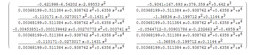
For this problem, this was done using symbolic algebra using the following steps, and the resulting \(G\left ( s\right ) \) matrix found is shown below
Using Matlab, the same procedure was done using syms as follows
And the output is
Generating the transfer function when aileron \(\delta _{a}=\SI{6}{\degree }\) is the input Transfer function \(G_{v,\delta _{a}}\)
\(G_{ij}\) is now found. The input is \(\delta _{a}\) which is \(j=1\). The output is \(v\), which is \(i=1\). Therefore \[ G_{11}\left ( s\right ) =G_{v,\delta _{a}}=\frac{\overset{N_{v,\delta _{a}}}{\overbrace{-2.89553s^{2}-6.54202s-0.621998}}}{s^{4}+0.6358s^{3}+0.938762s^{2}+0.511384s+0.00368199}\]
The side velocity \(v\) response to \(\delta _{a}=6^{o}\) is generated using Matlab


Transfer function \(G_{p,\delta _{a}}\)
The input now is \(\delta _{a}\) which is \(j=1\). The output is \(p\), which is \(i=2\). Therefore \[ G_{21}\left ( s\right ) =G_{p,\delta _{a}}=\frac{ \overbrace{-0.1431s^{3}-0.0273017s^{2}-0.110171s}^{N_{p,\delta _{a}}} }{s^{4}+0.6358s^{3}+0.938762s^{2}+0.511384s+0.00368199}\]
The roll rate \(p\) response to \(\delta _{a}=6^{o}\) is generated using Matlab

The bode plot for \(G_{p,\delta _{a}}\) is

Using transfer function \(G_{r,\delta _{a}}\)
The input now is \(\delta _{a}\) which is \(j=1\). The output is \(r\) which is \(i=3\). Therefore \[ G_{31}\left ( s\right ) =G_{r,\delta _{a}}=\frac{ \overbrace{-0.003741s^{3}+0.00270772s^{2}+0.000139442s-0.00453851}^{ N_{r,\delta _{a}}} }{s^{4}+0.6358s^{3}+0.938762s^{2}+0.511384s+0.00368199}\]
The yaw rate \(r\) response to \(\delta _{a}=6^{o}\) is generated using Matlab

The bode plot for \(G_{r,\delta _{a}}\) is now generated. This can be compared to figure 7.27(e) on page 250.

Transfer function \(G_{\phi ,\delta _{a}}\)
The input now is \(\delta _{a}\) which is \(j=1\). The output is \(\phi \),which is \(i=4\). Therefore \[ G_{41}\left ( s\right ) =G_{\phi ,\delta _{a}}=\frac{\overset{N_{\phi ,\delta _{a}}}{\overbrace{-0.1431s^{2}-0.0273017s-0.110171}}}{s^{4}+0.6358s^{3}+0.938762s^{2}+0.511384s+0.00368199}\]
The Euler angle \(\Phi \) response to \(\delta _{a}=\SI{6}{\degree }\) is found using Matlab

The bode plot for \(G_{\Phi ,\delta _{a}}\) is generated. This can be compared to figure 7.27(c) on page 249.

Generating the transfer function when rudder \(\delta _{r}=3^{o}\) is the input Transfer function \(G_{v,\delta r}\)
The input now is \(\delta _{r}\) which is \(j=2\). The output is \(v\) which is \(i=1\). Therefore \[ G_{12}\left ( s\right ) =G_{v,\delta _{r}}=\frac{ \overbrace{-5.642s^{3}+379.359s^{2}+167.893s-5.9341}^{N_{v,\delta _{r}}} }{s^{4}+0.6358s^{3}+0.938762s^{2}+0.511384s+0.00368199}\]
The lateral speed \(v\) response (side slip rate) to \(\delta _{r}=\SI{3}{\degree }\) is generated using Matlab

Bode plot for \(G_{v,\delta _{r}}\) is now generated. This can be compared to figure 7.26(a) on page 245.

The input now is \(\delta _{r}\) which is \(j=2\). The output is \(p\) which is \(i=2\). Therefore \[ G_{22}\left ( s\right ) =G_{p,\delta _{r}}=\frac{ \overbrace{-0.1144s^{3}-0.199712s^{2}-1.36834s}^{N_{p,\delta _{r}}} }{s^{4}+0.6358s^{3}+0.938762s^{2}+0.511384s+0.00368199}\] The roll rate \(p\) respones to \(\delta _{r}=3^{o}\) is generated using Matlab

Bode plot for \(G_{p,\delta _{r}}\) is now generated

Using transfer function \(G_{r,\delta r}\)
The input now is \(\delta _{r}\) which is \(j=2\). The output is \(r\) which is \(i=3\). Therefore \[ G_{32}\left ( s\right ) =G_{r,\delta _{r}}=\frac{ \overbrace{-0.4859s^{3}-0.232663s^{2}-0.00901786s-0.0564712}^{N_{r,\delta _{r}}} }{s^{4}+0.6358s^{3}+0.938762s^{2}+0.511384s+0.00368199}\]
The yaw rate \(r\) respones to \(\delta _{r}=3^{o}\) is generated using Matlab

The bode plot for \(G_{r,\delta _{r}}\) is now generated.

Using transfer function \(G_{\phi ,\delta _{r}}\)
The input now is \(\delta _{r}\) which is \(j=2\). The output is \(\phi \) which is \(i=4\). Therefore \[ G_{42}\left ( s\right ) =G_{\phi ,\delta _{r}}=\frac{\overset{N_{\phi ,\delta _{r}}}{\overbrace{-0.1144s^{2}-0.199712s-1.36834}}}{s^{4}+0.6358s^{3}+0.938762s^{2}+0.511384s+0.00368199}\]
The Euler angle \(\Phi \) respones to \(\delta _{r}=3^{o}\) is generated using Matlab

The bode plot for \(G_{\Phi ,\delta _{r}}\) is now generated. This can be compared to figure 7.26(c) on page 246.

Simultaneous response for aileron and rudder input \(\left ( \delta _{a}=6^{o},\delta _{r}=-3^{o}\right ) \) The transfer functions are found above. They are used to find the combined response. As was done for the longitudinal case, since the system is linear, the response to \(\delta _{a}=6^{o}\) is found and added to the response to \(\delta _{r}=\SI{-3}{\degree }\) to obtain the combined response.
Lateral \(v\) response to combined \(\left ( \delta _{a}=6^{o},\delta _{r}=-3^{o}\right ) \)

Yaw rate \(r\) response to combined \(\left ( \delta _{a}=6^{o},\delta _{r}=-3^{o}\right ) \)

Euler angle \(\Phi \) response to combined \(\left ( \delta _{a}=6^{o},\delta _{r}=-3^{o}\right ) \)

Simultaneous response for aileron and rudder input \(\left ( \delta _{a}=6^{o},\delta _{r}=+3^{o}\right ) \) The transfer functions are found above. They are used to obtain the combined response. As was done for the longitudinal case, since the system is linear, the response to \(\delta _{a}=6^{0}\) was added to the response to \(\delta _{r}=3^{o}\) to obtain the combined response.
Lateral \(v\) response to combined \(\left ( \delta _{a}=6^{o},\delta _{r}=+3^{o}\right ) \)

Yaw rate \(r\) response to combined \(\left ( \delta _{a}=6^{o},\delta _{r}=+3^{o}\right ) \)

Euler angle \(\Phi \) response to combined \(\left ( \delta _{a}=6^{o},\delta _{r}=+3^{o}\right ) \)
