
SOLUTION:
\[ G\left ( s\right ) =\frac{Ks+1}{s^{3}+s^{2}+\left ( K+k\right ) s+1}\]
For \(K=1\) the above becomes\[ G\left ( s\right ) =\frac{s+1}{s^{3}+s^{2}+\left ( 1+k\right ) s+1}\] Hence\begin{align*} S_{k}^{G} & =\frac{dG}{dk}\frac{k}{G}\\ & =\frac{d}{dk}\frac{s+1}{s^{3}+s^{2}+\left ( 1+k\right ) s+1}\left ( \frac{k}{\frac{s+1}{s^{3}+s^{2}+\left ( 1+k\right ) s+1}}\right ) \\ & =\frac{-s\left ( s+1\right ) }{\left ( s+ks+s^{2}+s^{3}+1\right ) ^{2}}\frac{k\left ( s^{3}+s^{2}+\left ( 1+k\right ) s+1\right ) }{s+1}\\ & =\frac{-ks}{1+\left ( 1+k\right ) s+s^{2}+s^{3}} \end{align*}
At nominal \(k=2\) the above becomes\[ \left . S_{k}^{G}\right \vert _{k=2}=\frac{-2s}{3s+s^{2}+s^{3}+1}\] Let \(s=j\omega \) then\[ S_{k}^{G}=\frac{-2\left ( j\omega \right ) }{3j\omega +\left ( j\omega \right ) ^{2}+\left ( j\omega \right ) ^{3}+1}=\frac{-2j\omega }{j\left ( 3\omega -\omega ^{3}\right ) +\left ( 1-\omega ^{2}\right ) }\] Taking the magnitude \[ \left \vert S_{k}^{G}\right \vert =\frac{2\omega }{\sqrt{\left ( 1-\omega ^{2}\right ) ^{2}+\left ( 3\omega -\omega ^{3}\right ) ^{2}}}\] Here is a plot of \(\left \vert S_{k}^{G}\right \vert \) as function of \(\omega \)

For \(K=100\) the transfer function becomes\begin{align*} G\left ( s\right ) & =\frac{Ks+1}{s^{3}+s^{2}+\left ( K+k\right ) s+1}\\ & =\frac{100s+1}{s^{3}+s^{2}+\left ( 100+k\right ) s+1} \end{align*}
Hence\begin{align*} S_{k}^{G} & =\frac{dG}{dk}\frac{k}{G}\\ & =\frac{d}{dk}\frac{100s+1}{s^{3}+s^{2}+\left ( 100+k\right ) s+1}\left ( \frac{k}{\frac{100s+1}{s^{3}+s^{2}+\left ( 100+k\right ) s+1}}\right ) \\ & =\frac{-s\left ( 100s+1\right ) }{\left ( 100s+ks+s^{2}+s^{3}+1\right ) ^{2}}\frac{k\left ( s^{3}+s^{2}+\left ( 100+k\right ) s+1\right ) }{100s+1}\\ & =\frac{-ks}{100s+ks+s^{2}+s^{3}+1} \end{align*}
At nominal \(k=2\) the above becomes\begin{align*} \left . S_{k}^{G}\right \vert _{k=2} & =\frac{-2s}{100s+2s+s^{2}+s^{3}+1}\\ & =\frac{-2s}{102s+s^{2}+s^{3}+1} \end{align*}
Let \(s=j\omega \) then\begin{align*} S_{k}^{G} & =\frac{-2\left ( j\omega \right ) }{102j\omega +\left ( j\omega \right ) ^{2}+\left ( j\omega \right ) ^{3}+1}\\ & =\frac{-2j\omega }{102j\omega -\omega ^{2}-j\omega ^{3}+1}\\ & =\frac{-2j\omega }{j\left ( 102\omega -\omega ^{3}\right ) +\left ( 1-\omega ^{2}\right ) } \end{align*}
Taking the magnitude\[ \left \vert S_{k}^{G}\right \vert =\frac{2\omega }{\sqrt{\left ( 1-\omega ^{2}\right ) ^{2}+\left ( 102\omega -\omega ^{3}\right ) ^{2}}}\] Here is a plot of \(\left \vert S_{k}^{G}\right \vert \) as function of \(\omega \)

We clearly see that as \(K\) became much larger, resonance occurs near \(\omega =10\). This shows that sensitivity of transfer function to changes in \(k\), depends on the value of \(K\).


SOLUTION:

From the above we see that
\begin{equation} Y=N\left ( x\right ) \tag{1} \end{equation}
The plot of \(Y\left ( x\right ) \) is given below based on the definition given in the problem

At the output of the controller we have\begin{align} x & =k\left ( R-N\left ( x\right ) \right ) \nonumber \\ x & =k\left ( R-Y\right ) \nonumber \\ x & =kR-kY\nonumber \\ Y & =R-\frac{x}{k} \tag{2} \end{align}
Equations (1) and (2) must both hold. We now setup a table of \(R\) and corresponding \(Y\) values, and using \(k=1\) for this part, we obtain
| \(R\) | \(Y=R-x\) | solution of \(Y=N\left ( x\right ) \) | \(Y\) at solution |
| \(0\) | \(-x\) | \(x=0\) | \(0\) |
| \(0.1\) | \(0.1-x\) | \(x=0\) | \(0\) |
| \(0.2\) | \(0.2-x\) | \(\vdots \) | \(\vdots \) |
| see program | \(\vdots \) | \(\vdots \) | \(\vdots \) |
Small code was written to finish the above table, using \(R=-2\cdots 2\) range with increments of \(0.1\). Here is the generated table, followed by the plot

And plot of \(Y\) vs. \(R\) is below

This below is the above plot, but with the original device output without feedback, in order to better see the effect of feedback with \(k=1\).

For \(k=1\), the dead zone did not change. But the slope became small after \(x=\pm 1\)
When \(r\left ( t\right ) =5\sin \left ( t\right )\), the following table shows result for \(t=-2\dots 2\).

the following is the plot of the output with the feedback for \(k=1\)

Matlab code to plot the solution
Now \(k=10,\) and part(b) was repeated. the following table shows result for \(t=-2\dots 2\).

And the following is the plot of the result

The above plot shows that with \(k=10\), the dead zone has shrunk to almost zero, and the output of the nonlinear device is now linear. This is good. This is another plot, for larger range of input values.

As range of input values become large, the output of the feedback linear device approaches the open loop device output. This is outside the dead zone region as can be seen from the above. Very close to the origin, there is very small non-linearity remains, but it is hard to see.
When the gain \(k\) is in the feedback loop, as shown in the following diagram

Therefore \begin{align*} x & =R-kY\\ Y & =\frac{\left ( R-x\right ) }{k} \end{align*}
Before, when the gain was in the feedforward, \(Y=R-\frac{x}{k}\), so now \(k\) affects \(R\) as well. Using this new \(x\), the above plot was reproduced for the case of \(r\left ( t\right ) =5\sin \left ( t\right ) \).
the following table shows result for \(t=-2\dots 2\).

And the following is the plot

We see the effect of reducing \(R\) (since it is now divided by \(k>1\)) and the output from the non-linear device is not as good as when the gain was in the feedforward. The dead zone has returned back and the output after the dead zone is much smaller in amplitude than the original open loop output. Putting the gain in the feedback loop does not appear to be a good choice in this case.

SOLUTION:
The first step is to convert the block diagram to signal flow diagram. By assigning variables as shown below, the following signal diagram we drawn
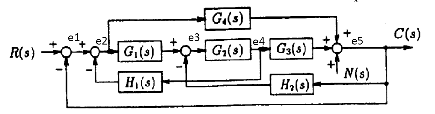
Converted to signal flow as

For finding \(\frac{C\left ( s\right ) }{R\left ( s\right ) }\,\ \) then \(N\left ( s\right ) \) is set to zero. There are two forward paths from \(R\left ( s\right ) \) to \(C\left ( s\right ) \) they are\begin{align*} M_{1} & =\left \{ 1,1,G_{1},G_{2},G_{3},1\right \} =G_{1}G_{2}G_{3}\\ M_{2} & =\left \{ 1,1,G_{4},1\right \} =G_{4} \end{align*}
The corresponding Mason deltas are\begin{align*} \Delta _{1} & =1\\ \Delta _{2} & =1-\left ( G_{2}\right ) \left ( -1\right ) =1+G_{2} \end{align*}
The loops, one at a time are\begin{align*} L_{1} & =\left ( G_{2}\right ) \left ( -1\right ) ,\left ( G_{1}\right ) \left ( G_{2}\right ) \left ( -H_{1}\right ) ,\left ( G_{2}\right ) \left ( G_{3}\right ) \left ( -H_{2}\right ) ,\left ( 1\right ) \left ( G_{1}\right ) \left ( G_{2}\right ) \left ( G_{3}\right ) \left ( 1\right ) \left ( -1\right ) ,\left ( G_{4}\right ) \left ( 1\right ) \left ( -1\right ) \\ & =-G_{2},-G_{1}G_{2}H_{1},-H_{2}G_{2}G_{3},-G_{1}G_{2}G_{3},-G_{4} \end{align*}
Two at a time are\begin{align*} L_{2} & =\left \{ \left ( G_{2}\right ) \left ( -1\right ) \times \left ( G_{4}\right ) \left ( 1\right ) \left ( -1\right ) \left ( 1\right ) \right \} \\ & =G_{2}G_{4} \end{align*}
Hence\begin{align*} \Delta & =1-\sum \left ( -G_{2}-G_{1}G_{2}H_{1}-H_{2}G_{2}G_{3}-G_{1}G_{2}G_{3}-G_{4}\right ) +\sum G_{2}G_{4}\\ & =1+G_{2}+G_{1}G_{2}H_{1}+H_{2}G_{2}G_{3}+G_{1}G_{2}G_{3}+G_{4}+G_{2}G_{4} \end{align*}
Hence \begin{align*} \frac{C\left ( s\right ) }{R\left ( s\right ) } & =\frac{\sum M_{i}\Delta _{i}}{\Delta }\\ & =\frac{G_{1}G_{2}G_{3}\left ( 1\right ) +G_{4}\left ( 1+G_{2}\right ) }{1+G_{2}+G_{1}G_{2}H_{1}+H_{2}G_{2}G_{3}+G_{1}G_{2}G_{3}+G_{4}+G_{2}G_{4}} \end{align*}
Hence\[ \fbox{$\frac{C\left ( s\right ) }{R\left ( s\right ) }=\frac{G_1G_2G_3+G_4+G_4G_2}{1+G_2+G_1G_2H_1+H_2G_2G_3+G_1G_2G_3+G_4+G_2G_4}$}\] For finding \(\frac{C\left ( s\right ) }{N\left ( s\right ) }\,\ \) then \(R\left ( s\right ) \) is set to zero. There is now one forward path from \(N\left ( s\right ) \) to \(C\left ( s\right ) \) \[ M_{1}=\left \{ 1,1\right \} =1 \] The corresponding Mason deltas are\[ \Delta _{1}=1-\left \{ \left ( G_{2}\right ) \left ( -1\right ) +\left ( G_{1}\right ) \left ( G_{2}\right ) \left ( -H_{1}\right ) \right \} =1+G_{2}+G_{1}G_{2}H_{1}\] The loops remain the same as above. Hence the mason delta do not change. Therefore\begin{align*} \frac{C\left ( s\right ) }{N\left ( s\right ) } & =\frac{\sum M_{i}\Delta _{i}}{\Delta }\\ & =\frac{\left ( 1\right ) \left ( 1+G_{2}+G_{1}G_{2}H_{1}\right ) }{1+G_{2}+G_{1}G_{2}H_{1}+H_{2}G_{2}G_{3}+G_{1}G_{2}G_{3}+G_{4}+G_{2}G_{4}} \end{align*}
Hence\[ \fbox{$\frac{C\left ( s\right ) }{N\left ( s\right ) }=\frac{1+G_2+G_1G_2H_1}{1+G_2+G_1G_2H_1+H_2G_2G_3+G_1G_2G_3+G_4+G_2G_4}$}\]
Since \[ C\left ( s\right ) =\frac{1+G_{2}+G_{1}G_{2}H_{1}}{1+G_{2}+G_{1}G_{2}H_{1}+H_{2}G_{2}G_{3}+G_{1}G_{2}G_{3}+G_{4}+G_{2}G_{4}}N\left ( s\right ) \] Then we want \( 1+G_{2}+G_{1}G_{2}H_{1} =0\) or for the denominator \[ 1+G_{2}+G_{1}G_{2}H_{1}+H_{2}G_{2}G_{3}+G_{1}G_{2}G_{3}+G_{4}+G_{2}G_{4} \] to be very large. Both of these will cause \(C\left ( s\right ) \) to remain zero for any value of \(N\left ( s\right ) \). But since the denominator is the same as for \(\frac{C\left ( s\right ) }{R\left ( s\right ) }\) then making this very large will also affect \(\frac{C\left ( s\right ) }{R\left ( s\right ) }\) which we do not want to. Hence the choice left is\[ 1+G_{2}+G_{1}G_{2}H_{1} =0 \]

SOLUTION:
For the \(\frac{Y_{7}}{Y_{1}}\), There are two forward paths. The following diagrams shows them with the gain on each.

\begin{align*} F_{1} & =G_{1}G_{2}G_{3}G_{4}G_{5}\\ F_{2} & =G_{6}G_{5} \end{align*}
Now \(\Delta _{k}\) is found for each forward loop. \(\Delta _{k}\) is the Mason \(\Delta \) but with \(F_{k}\) removed from the graph. Removing \(F_{1}\) removes all the loops, hence \[ \Delta _{1}=1 \] When removing \(F_{2}\) what remains is \(L_{2}\) and \(L_{3}\), hence \begin{align*} \Delta _{2} & =1-\left ( L_{2}+L_{3}\right ) \\ & =1-\left ( -H_{2}G_{2}-H_{3}G_{3}\right ) \\ & =1+\left ( H_{2}G_{2}+H_{3}G_{3}\right ) \end{align*}
For the \(\frac{Y2}{Y_{1}}\), there is one forward path \(F_{1}=1\), the associated \(\Delta _{1}\) is\begin{align*} \Delta _{1} & =1-\sum -G_{2}H_{2}-G_{3}H_{3}-G_{4}G_{5}H_{4}-H_{6}-G_{2}G_{3}G_{4}G_{5}H_{5}\\ & +\sum \left ( -G_{2}H_{2}\right ) \left ( -G_{4}G_{5}H_{4}\right ) +\left ( -G_{2}H_{2}\right ) \left ( -H_{6}\right ) +\left ( -G_{3}H_{3}\right ) \left ( -H_{6}\right ) \\ & =1+\overbrace{G_{2}H_{2}+G_{3}H_{3}+G_{4}G_{5}H_{4}+H_{6}+G_{2}G_{3}G_{4}G_{5}H_{5}}^{\text{one at a time}} + \overbrace{G_{2}H_{2}G_{4}G_{5}H_{4}+G_{2}H_{2}H_{6}+G_{3}H_{3}H_{6}}^{\text{two at a time}} \end{align*}
There are 8 loops. The following diagrams shows the loops with the gains

\begin{align*} \Delta & =1-\left ( L_{1}+L_{2}+L_{3}+L_{4}+L_{5}+L_{6}+L_{7}+L_{8}\right ) \\ & +\left ( L_{1}L_{3}+L_{1}L_{4}+L_{1}L_{6}+L_{2}L_{4}+L_{2}L_{6} +L_{3} L_{6}+L_{3}L_{7}\right ) -L_{1}L_{3}L_{6}\\ \end{align*}
Therefore\begin{align} \Delta & =1+\overbrace{H_{1}G_{1}+H_{2}G_{2}+H_{3}G_{3}+H_{4}G_{4}G_{5}+H_{5}G_{2}G_{3}G_{4}G_{5}+H_{6}-G_{5}G_{6}H_{1}H_{5}-G_{6}G_{5}H_{4}H_{3}H_{2}H_{1}}^{\text{one at a time}} \tag{1}\\ & +\overbrace{\left ( H_{1}G_{1}H_{3}G_{3}+H_{1}G_{1}H_{4}G_{4}G_{5}+H_{1}H_{6}G_{1}+H_{2}G_{2}H_{4}G_{4}G_{5}+H_{2}G_{2}H_{6}+H_{3}G_{3}H_{6}-G_{3}H_{3}G_{6}G_{5}H_{5}H_{1}\right ) }^{\text{two at time}} \nonumber \\ & +\overbrace{H_{1}G_{1}H_{3}G_{3}H_{6}}^{\text{three at time}}\nonumber \end{align}
For \(G\left ( s\right ) =\frac{Y_{7}}{Y_{1}}\), and using result found above in part (a) and part (b)\begin{align*} G\left ( s\right ) & =\frac{Y_{7}}{Y_{1}}\\ & =\frac{\Delta _{1}F_{1}+\Delta _{2}F_{2}}{\Delta }\\ & =\frac{\left ( G_{1}G_{2}G_{3}G_{4}G_{5}\right ) +G_{6}G_{5}\left ( 1+H_{2}G_{2}+H_{3}G_{3}\right ) }{\Delta } \end{align*}
Where \(\Delta \) is given in (1) found in part(b). To obtain \(\frac{Y_{2}}{Y_{1}}\)
\begin{align*} \x & =\frac{\Delta _{1}F_{1}}{\Delta }\\ & =\frac{\e }{\Delta }\\ & =\frac{1+\y +\z }{\Delta } \end{align*}
 ;
;
 ;
;
 ;
;
 ;
;
 ;
;