
Obtain two distinct Laurent expansions for \(f\left ( z\right ) =\frac{3z+1}{z^{2}-1}\) around \(z=1\) and tell where each converges.
Solution
\(f\left ( z\right ) \) has singularities at \(z=\pm 1\) and the expansion is around one of these singularities. Looking at the diagram
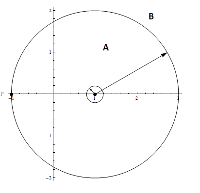
For \(\frac{2}{z-1}\), since its pole is at \(z=1\) and so we expand outwards, and hence it is already in form of Laurent series around \(z=1\), and for \(\frac{1}{z+1}\) since its pole is at \(z=-1\), hence we expand inwards, and so it is expanded in Taylor series\[ f\left ( z\right ) =\overset{Laurent}{\overbrace{\frac{2}{z-1}}}+\overset{Taylor}{\overbrace{\frac{1}{z+1}}}\] Looking at the second term above, expand in Taylor series\begin{align*} \frac{1}{z+1} & =\frac{1}{\left ( z-1\right ) +1+1}=\frac{1}{\left ( z-1\right ) +2}=\frac{1}{2}\frac{1}{1+\frac{1}{2}\left ( z-1\right ) }\\ & =\frac{1}{2}\sum \limits _{n=0}^{\infty }\left ( -1\right ) ^{n}\left ( \frac{1}{2}\right ) ^{n}\left ( z-1\right ) ^{n}\qquad \left \vert z-1\right \vert <2 \end{align*}
Therefore, for region A\begin{align*} f\left ( z\right ) & =\frac{2}{z-1}+\frac{1}{2}\sum \limits _{n=0}^{\infty }\left ( -1\right ) ^{n}\left ( \frac{1}{2}\right ) ^{n}\left ( z-1\right ) ^{n}\\ & =\frac{2}{z-1}+\frac{1}{2}\left ( 1-\frac{1}{2}\left ( z-1\right ) +\frac{1}{4}\left ( z-1\right ) ^{2}-\frac{1}{16}\left ( z-1\right ) ^{3}+\cdots \right ) \\ & =\frac{2}{z-1}+\frac{1}{2}-\frac{1}{4}\left ( z-1\right ) +\frac{1}{8}\left ( z-1\right ) ^{2}-\frac{1}{16}\left ( z-1\right ) ^{3}+\cdots \end{align*}
This is valid for \(0<\left \vert z-1\right \vert <2,z\neq 1\)
Region B
This is the region outside the large circle to infinity. Since expanding outwards, both terms will use Laurent series now.\[ f\left ( z\right ) =\overset{Laurent}{\overbrace{\frac{2}{z-1}}}+\overset{Laurent}{\overbrace{\frac{1}{z+1}}}\] \(\frac{2}{z-1}\) is already in Laurent series, for the second term\begin{align*} \frac{1}{z+1} & =\frac{1}{\left ( z-1\right ) +1+1}=\frac{1}{\left ( z-1\right ) +2}=\frac{1}{\left ( z-1\right ) }\frac{1}{1+\frac{2}{z-1}}\\ & =\frac{1}{\left ( z-1\right ) }\sum \limits _{n=0}^{\infty }\left ( -1\right ) ^{n}\frac{2^{n}}{\left ( z-1\right ) ^{n}}\qquad \left \vert z-1\right \vert >2 \end{align*}
Hence\begin{align*} f\left ( z\right ) & =\frac{2}{z-1}+\frac{1}{\left ( z-1\right ) }\sum \limits _{n=0}^{\infty }\left ( -1\right ) ^{n}\frac{2^{n}}{\left ( z-1\right ) ^{n}}\\ & =\frac{2}{z-1}+\frac{1}{\left ( z-1\right ) }\left ( 1-\frac{2}{\left ( z-1\right ) }+\frac{4}{\left ( z-1\right ) ^{2}}-\frac{8}{\left ( z-1\right ) ^{3}}+\cdots \right ) \\ & =\frac{2}{z-1}+\frac{1}{z-1}-\frac{2}{\left ( z-1\right ) ^{2}}+\frac{4}{\left ( z-1\right ) ^{3}}-\frac{8}{\left ( z-1\right ) ^{4}}+\cdots \\ & =\frac{3}{z-1}-\frac{2}{\left ( z-1\right ) ^{2}}+\frac{4}{\left ( z-1\right ) ^{3}}-\frac{8}{\left ( z-1\right ) ^{4}}+\cdots \end{align*}
This is valid for \(\left \vert z-1\right \vert >2\)
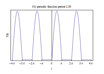
Find the Fourier expansion of the periodic function whose definition on one period is
\[ f\left ( t\right ) =\left \{ \begin{array} [c]{ccc}0 & & -\pi \leq t\leq 0\\ \sin t & & 0\leq t\leq \pi \end{array} \right . \]
Solution
Hence\begin{align*} c_{n} & =\frac{1}{2\pi }\left ( \int \limits _{-\pi }^{0}f\left ( t\right ) e^{-int}dt+\int \limits _{0}^{\pi }f\left ( t\right ) e^{-int}dt\right ) \\ & =\frac{1}{2\pi }\int \limits _{0}^{\pi }\sin \left ( t\right ) e^{-int}dt \end{align*}
Integration by parts, \(\int udv=uv-\int vdu\), let \(u=\sin \left ( t\right ) \rightarrow du=\cos \left ( t\right ) \) and \(dv=e^{-int}\rightarrow v=\frac{e^{-int}}{-in}\), therefore\begin{align*} I & =\left [ uv\right ] _{0}^{\pi }-\int \limits _{0}^{\pi }vdu\\ & =\left [ \sin \left ( t\right ) \frac{e^{-int}}{-in}\right ] _{0}^{\pi }-\int \limits _{0}^{\pi }\cos \left ( t\right ) \frac{e^{-int}}{-in}dt\\ & =\overset{0}{\overbrace{\left [ \sin \left ( \pi \right ) \frac{e^{-in\pi }}{-in}-\sin \left ( 0\right ) \frac{e^{-in0}}{-in}\right ] _{0}^{\pi }}}+\frac{1}{in}\int \limits _{0}^{\pi }\cos \left ( t\right ) e^{-int}dt\\ & =\frac{1}{in}\int \limits _{0}^{\pi }\cos \left ( t\right ) e^{-int}dt \end{align*}
Integration by parts again, \(\int udv=uv-\int vdu\), let \(u=\cos \left ( t\right ) \rightarrow du=-\sin \left ( t\right ) \) and \(dv=e^{-int}\rightarrow v=\frac{e^{-int}}{-in}\), therefore\begin{align*} I & =\frac{1}{in}\left ( \left [ \cos \left ( t\right ) \frac{e^{-int}}{-in}\right ] _{0}^{\pi }-\int \limits _{0}^{\pi }-\sin \left ( t\right ) \frac{e^{-int}}{-in}dt\right ) \\ & =\frac{1}{in}\left ( \left [ \cos \left ( \pi \right ) \frac{e^{-in\pi }}{-in}-\cos \left ( 0\right ) \frac{e^{-in0}}{-in}\right ] -\frac{1}{in}\int \limits _{0}^{\pi }\sin \left ( t\right ) e^{-int}dt\right ) \\ & =\frac{1}{in}\left ( \left [ \frac{e^{-in\pi }}{in}+\frac{1}{in}\right ] -\frac{1}{in}\int \limits _{0}^{\pi }\sin \left ( t\right ) e^{-int}dt\right ) \end{align*}
But \(e^{-in\pi }=\cos n\pi -i\sin n\pi =\left ( -1\right ) ^{n}\) for integer \(n\), hence\begin{align*} I & =\frac{1}{in}\left ( \frac{\left ( -1\right ) ^{n}+1}{in}-\frac{1}{in}\int \limits _{0}^{\pi }\sin \left ( t\right ) e^{-int}dt\right ) \\ & =\frac{\left ( -1\right ) ^{n}+1}{-n^{2}}+\frac{1}{n^{2}}\int \limits _{0}^{\pi }\sin \left ( t\right ) e^{-int}dt \end{align*}
But \(\int \limits _{0}^{\pi }\sin \left ( t\right ) e^{-int}dt\) in the RHS above is \(I\) itself. Hence solving for \(I\) gives\begin{align*} I & =\frac{\left ( -1\right ) ^{n}+1}{-n^{2}}+\frac{1}{n^{2}}I\\ I\left ( 1-\frac{1}{n^{2}}\right ) & =\frac{\left ( -1\right ) ^{n}+1}{-n^{2}}\\ I\left ( \frac{n^{2}-1}{n^{2}}\right ) & =\frac{\left ( -1\right ) ^{n}+1}{-n^{2}}\\ I & =\frac{\left ( -1\right ) ^{n}+1}{-n^{2}}\frac{n^{2}}{n^{2}-1}\\ & =\frac{\left ( -1\right ) ^{n}+1}{1-n^{2}} \end{align*}
Therefore \begin{align*} c_{n} & =\frac{1}{2\pi }I\\ & =\frac{\left ( -1\right ) ^{n}+1}{2\pi \left ( 1-n^{2}\right ) } \end{align*}
And hence \begin{align*} \tilde{f}\left ( t\right ) & =\sum \limits _{n=-\infty }^{\infty }c_{n}e^{int}\\ & =\sum \limits _{n=-\infty }^{\infty }\frac{\left ( -1\right ) ^{n}+1}{2\pi \left ( 1-n^{2}\right ) }e^{int} \end{align*}
For \(c_{0}\)\[ c_{0}=\frac{1}{\pi }\] Looking at some terms, for \(n=1\) and \(n=-1\), there can not be substituted in the denominator since that will produce a division by \(0,\) hence L’hospital rule is used. Since \(-1=e^{i\pi \text{ }}\)then write \(-1^{n}=e^{i\pi n}\) to simplify taking derivatives.\[ \lim _{n->1}\frac{f\left ( n\right ) }{g\left ( n\right ) }=\lim _{n->1}\frac{f^{\prime }\left ( n\right ) }{g^{\prime }\left ( n\right ) }=\lim _{n->1}\frac{\frac{d}{dn}\left ( \left ( -1\right ) ^{n}+1\right ) }{\frac{d}{dn}\left ( 2\pi \left ( 1-n^{2}\right ) \right ) }=\lim _{n->1}\frac{i\pi e^{i\pi n}}{-4\pi n}=\frac{i\pi e^{i\pi }}{-4\pi }=\frac{-i\pi }{-4\pi }=\frac{i}{4}\] and\[ \lim _{n->-1}\frac{f\left ( n\right ) }{g\left ( n\right ) }=\lim _{n->-1}\frac{f^{\prime }\left ( n\right ) }{g^{\prime }\left ( n\right ) }=\lim _{n->-1}\frac{\frac{d}{dn}\left ( \left ( -1\right ) ^{n}+1\right ) }{\frac{d}{dn}\left ( 2\pi \left ( 1-n^{2}\right ) \right ) }=\lim _{n->-1}\frac{i\pi e^{i\pi n}}{-4\pi n}=\frac{i\pi e^{-i\pi }}{4\pi }=\frac{-i\pi }{4\pi }=\frac{-i}{4}\] For all other odd \(n,\) all terms cancel. This means that for \(n=\pm 3,\pm 5,\cdots \) all \(c_{n}\) terms are zero. For example, for \(n=3\) the term is \(c_{3}=\frac{\left ( -1\right ) ^{3}+1}{\pi \left ( 1-9\right ) }=0\) since all the numerators are zero for \(odd\) \(n\).
For all even \(n\), terms with \(n=\pm 2,\pm 4,\cdots \) are combined into one term as follows\begin{align*} n & =2\rightarrow c_{2}e^{int}=\frac{\left ( -1\right ) ^{n}+1}{2\pi \left ( 1-n^{2}\right ) }e^{int}=\frac{\left ( -1\right ) ^{2}+1}{2\pi \left ( 1-4\right ) }e^{i2t}=\frac{1}{-3\pi }e^{i2t}\\ n & =-2\rightarrow c_{-2}e^{int}=\frac{\left ( -1\right ) ^{n}+1}{2\pi \left ( 1-n^{2}\right ) }e^{int}=\frac{\left ( -1\right ) ^{-2}+1}{2\pi \left ( 1-4\right ) }e^{-i2t}=\frac{1}{-3\pi }e^{-i2t} \end{align*}
Hence\[ c_{2}e^{i2t}+c_{-2}e^{-2it}=\frac{1}{-3\pi }\left ( e^{i2t}+e^{-2it}\right ) =\frac{2}{-3\pi }\cos \left ( 2t\right ) \] The same for all other even \(n.\) Therefore, all the \(odd\) \(n\) terms vanish other than for \(n=\pm 1\) and all the even values produce a cosine terms. Hence\begin{align*} \tilde{f}\left ( t\right ) & =\overset{c_{0}}{\overbrace{\frac{1}{\pi }}}+\overset{c_{1}e^{it}+c_{-1}e^{-it}}{\overbrace{\left ( \frac{i}{4}e^{it}+\frac{-i}{4}e^{-it}\right ) }}+\sum \limits _{n=2,4,6,\cdots }^{\infty }\frac{2}{2\pi \left ( 1-n^{2}\right ) }\left ( e^{int}+e^{-int}\right ) \\ & =\frac{1}{\pi }+\frac{1}{2}\left ( \frac{-1}{2i}e^{-it}+\frac{1}{2i}e^{it}\right ) +\frac{2}{\pi }\sum \limits _{n=2,4,6,\cdots }^{\infty }\frac{\cos nt}{\left ( 1-n^{2}\right ) }\\ & =\frac{1}{\pi }+\frac{1}{2}\left ( \frac{e^{it}-e^{-it}}{2i}\right ) +\frac{2}{\pi }\sum \limits _{n=2,4,6,\cdots }^{\infty }\frac{\cos nt}{\left ( 1-n^{2}\right ) } \end{align*}
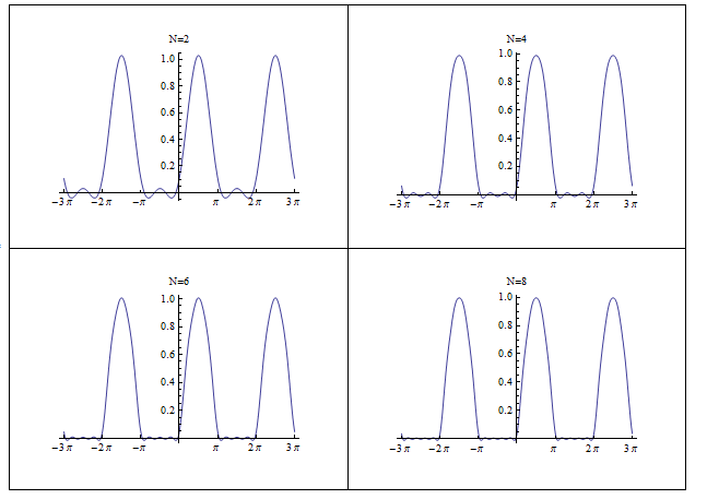
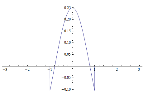
But \(\left ( \frac{e^{it}-e^{-it}}{2i}\right ) =\sin t\) hence\[ \tilde{f}\left ( t\right ) =\frac{1}{2}\sin \left ( t\right ) +\frac{1}{\pi }+\frac{2}{\pi }\sum \limits _{n=2,4,6,\cdots }^{\infty }\frac{\cos nt}{\left ( 1-n^{2}\right ) }\] Therefore\[ \tilde{f}\left ( t\right ) =\frac{1}{2}\sin \left ( t\right ) +\frac{1}{\pi }+\frac{2}{\pi }\frac{\cos 2t}{-3}+\frac{2}{\pi }\frac{\cos 4t}{-15}+\frac{2}{\pi }\frac{\cos 6t}{-35}+\cdots \] To verify this is correct, here is a plot of the Fourier series approximation of \(f\left ( t\right ) \) for increasing number of terms.
Find the solution of \(y^{\prime \prime }+9y=f\left ( t\right ) ;y\left ( 0\right ) =y^{\prime }\left ( 0\right ) =0\) and \(f\left ( t\right ) =\left \vert t\right \vert \) for \(-\pi \leq t\leq \pi \)
solution
The function \(f\left ( t\right ) \) is
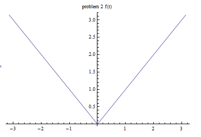
The problem did not say if this is one period of a periodic function of if the function is zero beyond the given range. I assumed it is periodic and hence using Fourier series to solve this.
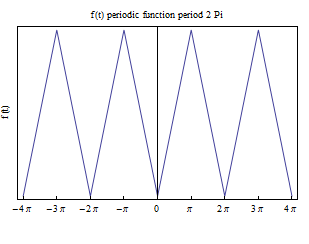
The period is therefore \(T=2\pi \) and using Fourier series gives\begin{align*} \tilde{f}\left ( t\right ) & =\sum \limits _{n=-\infty }^{\infty }c_{n}e^{int}\\ c_{n} & =\frac{1}{2\pi }\int _{-\pi }^{\pi }f\left ( t\right ) e^{-int}dt\\ & =\frac{1}{2\pi }\int _{-\pi }^{0}-te^{-int}dt+\frac{1}{2\pi }\int _{0}^{\pi }te^{-int}dt \end{align*}
For \(n=0,c_{0}=\frac{1}{2\pi }\int _{-\pi }^{0}-tdt+\frac{1}{2\pi }\int _{0}^{\pi }tdt=\frac{-1}{2\pi }\left [ \frac{t^{2}}{2}\right ] _{-\pi }^{0}+\frac{1}{2\pi }\left [ \frac{t^{2}}{2}\right ] _{0}^{\pi }=\frac{-1}{4\pi }\left [ 0-\left ( -\pi \right ) ^{2}\right ] +\frac{1}{4\pi }\left [ \pi ^{2}\right ] \), hence\begin{align*} c_{0} & =\frac{1}{4\pi }\pi ^{2}+\frac{1}{4\pi }\pi ^{2}\\ & =\frac{\pi }{2} \end{align*}
For other \(n\) values, Integrate by parts. For the first integral, \[ I_{1}=\frac{-1}{2\pi }\int _{-\pi }^{0}te^{-int}dt \] it becomes \(\int te^{-int}dt\Rightarrow \left [ uv\right ] -\int vdu\), let \(u=t,dv=e^{-int}\), hence \(du=1;v=\frac{e^{-int}}{-in}\) and \(\int te^{-int}dt=\left [ \frac{te^{-int}}{-in}\right ] +\frac{1}{in}\int e^{-int}dt\)
Therefore\begin{align*} I_{1} & =\frac{-1}{2\pi }\left ( \left [ \frac{te^{-int}}{-in}\right ] _{-\pi }^{0}+\frac{1}{in}\int _{-\pi }^{0}e^{-int}dt\right ) \\ & =\frac{-1}{2\pi }\left ( -\frac{1}{in}\left [ 0-\left ( -\pi e^{in\pi }\right ) \right ] +\frac{1}{in}\left [ \frac{e^{-int}}{-in}\right ] _{-\pi }^{0}\right ) \\ & =\frac{-1}{2\pi }\left ( \frac{-1}{in}\pi e^{in\pi }+\frac{1}{n^{2}}\left [ e^{-int}\right ] _{-\pi }^{0}\right ) \\ & =\frac{-1}{2\pi }\left ( \frac{-1}{in}\pi e^{in\pi }+\frac{1}{n^{2}}\left [ 1-e^{in\pi }\right ] \right ) \\ & =\frac{-1}{2\pi }\left ( \frac{-1}{in}\pi e^{in\pi }+\frac{1}{n^{2}}-\frac{1}{n^{2}}e^{in\pi }\right ) \end{align*}
For the second integral, \begin{align*} I_{2} & =\frac{1}{2\pi }\int _{0}^{\pi }te^{-int}dt\\ & =\frac{1}{2\pi }\left ( \left [ \frac{te^{-int}}{-in}\right ] _{0}^{\pi }+\frac{1}{in}\int _{0}^{\pi }e^{-int}dt\right ) \\ & =\frac{1}{2\pi }\left ( \frac{-1}{in}\left [ \pi e^{-in\pi }-0\right ] +\frac{1}{in}\left [ \frac{e^{-int}}{-in}\right ] _{0}^{\pi }\right ) \\ & =\frac{1}{2\pi }\left ( \frac{-1}{in}\pi e^{-in\pi }+\frac{1}{n^{2}}\left [ e^{-int}\right ] _{0}^{\pi }\right ) \\ & =\frac{1}{2\pi }\left ( \frac{-\pi e^{-in\pi }}{in}+\frac{1}{n^{2}}\left [ e^{-in\pi }-1\right ] \right ) \\ & =\frac{1}{2\pi }\left ( \frac{-\pi e^{-in\pi }}{in}+\frac{1}{n^{2}}e^{-in\pi }-\frac{1}{n^{2}}\right ) \end{align*}
Hence\begin{align*} c_{n} & =I_{1}+I_{2}\\ & =\frac{-1}{2\pi }\left ( \frac{-\pi e^{in\pi }}{in}+\frac{1}{n^{2}}-\frac{1}{n^{2}}e^{in\pi }\right ) +\frac{1}{2\pi }\left ( \frac{-\pi e^{-in\pi }}{in}+\frac{1}{n^{2}}e^{-in\pi }-\frac{1}{n^{2}}\right ) \\ & =\frac{1}{2\pi }\left ( \frac{\pi e^{in\pi }}{in}-\frac{1}{n^{2}}+\frac{1}{n^{2}}e^{in\pi }+\frac{-\pi e^{-in\pi }}{in}+\frac{1}{n^{2}}e^{-in\pi }-\frac{1}{n^{2}}\right ) \\ & =\frac{1}{2\pi }\left ( \frac{\pi }{n}\left ( \frac{e^{in\pi }}{i}-\frac{e^{-in\pi }}{i}\right ) +\frac{1}{n^{2}}\left ( e^{in\pi }+e^{-in\pi }\right ) -\frac{2}{n^{2}}\right ) \\ & =\frac{1}{2\pi }\left ( \frac{\pi }{n}\overset{0}{\overbrace{\left ( 2\sin n\pi \right ) }}+\frac{1}{n^{2}}\left ( 2\cos n\pi \right ) -\frac{2}{n^{2}}\right ) \\ & =\frac{1}{2\pi }\left ( \frac{1}{n^{2}}2\left ( -1\right ) ^{n}-\frac{2}{n^{2}}\right ) \\ & =\frac{1}{\pi n^{2}}\left ( -1^{n}-1\right ) \end{align*}
The above is for all \(n\) other than \(n=0\) where \(c_{0}=\) \(\frac{\pi }{2}\). The above shows that for \(c_{n}=0\) for even \(n\) and \(c_{n}=\frac{-2}{\pi n^{2}}\) for odd \(n\). Hence, by combining negative and positive \(n\)\begin{align*} \tilde{f}\left ( t\right ) & =\sum \limits _{n=-\infty }^{\infty }c_{n}e^{int}\\ & =\frac{\pi }{2}+\sum \limits _{\substack{n=-\infty \\odd\ n,n\neq 0}}^{\infty }\frac{-2}{\pi n^{2}}e^{int}\\ & =\frac{\pi }{2}+\sum \limits _{\substack{n=-\infty \\odd\ n,n\neq 0}}^{\infty }\frac{-2}{\pi n^{2}}e^{int} \end{align*}
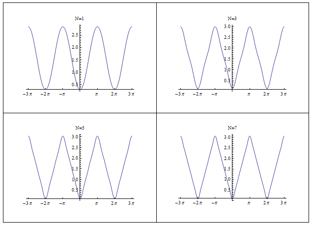
To verify, here is a plot showing the approximation
Therefore, the differential equation is\[ y^{\prime \prime }+9y=\frac{\pi }{2}+\sum \limits _{\substack{n=-\infty \\odd\ n,n\neq 0}}^{\infty }\frac{-2}{\pi n^{2}}e^{int}\] The homogeneous solution is now found\[ y_{h}^{\prime \prime }+9y_{h}=0 \] The characteristic polynomial is \(\lambda ^{2}+9=0\), hence \(\lambda =\pm i3\) and the solution is \[ y_{h}=A\cos 3t+B\sin 3t \] For \(y_{p}\), assume it has a Fourier series (using same frequency as forcing function, since linear system) \begin{align*} y_{p} & =C_{0}+\sum _{\substack{n=-\infty \\n\neq 0}}^{\infty }C_{n}e^{int}\\ y_{p}^{\prime } & =\sum _{\substack{n=-\infty \\n\neq 0}}^{\infty }inC_{n}e^{int}\\ y_{p}^{\prime \prime } & =\sum _{\substack{n=-\infty \\n\neq 0}}^{\infty }-n^{2}C_{n}e^{int} \end{align*}
Hence the DE becomes\[ \sum _{\substack{n=-\infty \\n\neq 0}}^{\infty }-n^{2}C_{n}e^{int}+9C_{0}+\sum _{\substack{n=-\infty \\n\neq 0}}^{\infty }9C_{n}e^{int}=\frac{\pi }{2}+\sum \limits _{\substack{n=-\infty \\odd\ n,n\neq 0}}^{\infty }\frac{-2}{\pi n^{2}}e^{int}\] For \(n=0\), \begin{align*} 9C_{0} & =\frac{\pi }{2}\\ C_{0} & =\frac{\pi }{18} \end{align*}
For all other \(n\) the terms can be combined as\begin{align*} \left ( -n^{2}C_{n}+9C_{n}\right ) & =\frac{-2}{\pi n^{2}}\\ C_{n} & =\frac{-2}{\left ( 9-n^{2}\right ) \pi n^{2}}\qquad n\neq 0,n\neq \pm 3,n\ odd \end{align*}
Notice that for \(n=\pm 3\) the above is not defined since the denominator becomes zero. So this term is not used (what else to do?)
Hence, \begin{align*} y_{p} & =\frac{\pi }{18}+\sum _{n=1,5,7,\cdots }^{\infty }\frac{-2}{\left ( 9-n^{2}\right ) \pi n^{2}}\left ( e^{int}+e^{-int}\right ) \\ & =\frac{\pi }{18}+\sum _{n=1,5,7,\cdots }^{\infty }\frac{-2}{\left ( 9-n^{2}\right ) \pi n^{2}}2\cos nt\\ & =\overset{n=0}{\overbrace{\frac{\pi }{18}}}\overset{n=1}{\overbrace{-\frac{1}{2\pi }\left ( \cos t\right ) }}-\frac{4}{\pi }\sum _{n=5,7,9,\cdots }^{\infty }\frac{1}{\left ( 9-n^{2}\right ) n^{2}}\cos nt\\ & =\frac{\pi }{18}-\frac{1}{2\pi }\cos t-\frac{4}{\pi }\sum _{n=5,7,9,\cdots }^{\infty }\frac{\cos nt}{\left ( 9-n^{2}\right ) n^{2}} \end{align*}
The final solution is\begin{align*} y & =y_{h}+y_{p}\\ & =A\cos 3t+B\sin 3t+\frac{\pi }{18}-\frac{1}{2\pi }\cos t-\frac{4}{\pi }\sum _{n=5,7,9,\cdots }^{\infty }\frac{\cos nt}{\left ( 9-n^{2}\right ) n^{2}} \end{align*}
Constants from initial conditions are now found\begin{align*} y\left ( 0\right ) & =0=A+\frac{\pi }{18}-\frac{1}{2\pi }-\frac{4}{\pi }\sum _{n=5,7,9,\cdots }^{\infty }\frac{1}{\left ( 9-n^{2}\right ) n^{2}}\\ A & =-\frac{\pi }{18}+\frac{2}{4\pi }-\frac{1}{\pi }\sum _{n=5,7,9,\cdots }^{\infty }\frac{-4}{\left ( 9-n^{2}\right ) n^{2}} \end{align*}
But, using CAS, found that \[ \sum _{n=5,7,9\cdots }^{\infty }\frac{-4}{\left ( 9-n^{2}\right ) n^{2}}=\frac{1}{162}\left ( 91-9\pi ^{2}\right ) \] Hence\begin{align*} A & =-\frac{\pi }{18}+\frac{2}{4\pi }-\frac{1}{\pi }\frac{1}{162}\left ( 91-9\pi ^{2}\right ) \\ & =-\frac{5}{81\pi } \end{align*}
Taking derivative of the general solution\[ y^{\prime }\left ( t\right ) =-3A\sin 3t+3B\cos 3t+\frac{\pi }{18}+\frac{2}{4\pi }\sin t+\frac{1}{\pi }\sum _{n=5,7,9,\cdots }^{\infty }\frac{4n\sin \left ( nt\right ) }{\left ( 9-n^{2}\right ) n^{2}}\] Using initial conditions \(y^{\prime }\left ( 0\right ) =0\)\[ 0=3B \] Hence \(B=0\), and solution is\[ y\left ( t\right ) =-\frac{5}{81\pi }\cos 3t+\frac{\pi }{18}-\frac{2}{4\pi }\cos t+\frac{1}{\pi }\sum _{n=5,7,9,\cdots }^{\infty }\frac{-4\cos \left ( nt\right ) }{\left ( 9-n^{2}\right ) n^{2}}\]
Find the Fourier transform of \(f\left ( t\right ) =\left \{ \begin{array} [c]{ccc}0 & & -\infty <t\leq 0\\ \sin \left ( t\right ) & & 0\leq t\leq \pi \\ 0 & & \pi \leq t<\infty \end{array} \right . \)
Solution
By definition \begin{align*} \mathcal{F}\left ( f\left ( t\right ) \right ) & =\int _{-\infty }^{\infty }f\left ( t\right ) e^{-i\omega t}dt\\ & =\int _{0}^{\pi }\sin \left ( t\right ) e^{-i\omega t}dt \end{align*}
Let \[ I=\int _{0}^{\pi }\sin \left ( t\right ) e^{-i\omega t}dt \] Integration by part \(\int udv\Rightarrow \left [ uv\right ] -\int vdu\), let \(u=\sin t,dv=e^{-i\omega t}\), hence \(du=\cos t;v=\frac{e^{-i\omega t}}{-i\omega }\) hence\begin{align*} I & =\left [ \sin t\frac{e^{-i\omega t}}{-i\omega }\right ] _{0}^{\pi }-\int \cos t\frac{e^{-i\omega t}}{-i\omega }dt\\ & =0+\frac{1}{i\omega }\int \cos te^{-i\omega t}dt\\ & =\frac{1}{i\omega }\int \cos te^{-i\omega t}dt \end{align*}
Integration by part \(\int udv\Rightarrow \left [ uv\right ] -\int vdu\), let \(u=\cos t,dv=e^{-i\omega t}\), hence \(du=-\sin t;v=\frac{e^{-i\omega t}}{-i\omega }\) hence\begin{align*} I & =\frac{1}{i\omega }\left ( \left [ \cos t\frac{e^{-i\omega t}}{-i\omega }\right ] _{0}^{\pi }-\frac{1}{i\omega }\overset{I}{\overbrace{\int \sin te^{-i\omega t}dt}}\right ) \\ & =\frac{1}{i\omega }\left ( \frac{-1}{i\omega }\left [ \cos te^{-i\omega t}\right ] _{0}^{\pi }-\frac{1}{i\omega }I\right ) \\ & =\frac{1}{i\omega }\left ( \frac{-1}{i\omega }\left [ \cos \pi e^{-i\omega \pi }-1\right ] -\frac{1}{i\omega }I\right ) \\ & =\frac{1}{\omega ^{2}}\left [ \cos \pi e^{-i\omega \pi }-1\right ] +\frac{1}{\omega ^{2}}I\\ I\left ( 1-\frac{1}{\omega ^{2}}\right ) & =\frac{1}{\omega ^{2}}\left [ \cos \pi e^{-i\omega \pi }-1\right ] \\ I\left ( \frac{\omega ^{2}-1}{\omega ^{2}}\right ) & =\frac{\cos \pi e^{-i\omega \pi }-1}{\omega ^{2}}\\ I & =\frac{\cos \pi e^{-i\omega \pi }-1}{\omega ^{2}-1}=\frac{-e^{-i\omega \pi }-1}{\omega ^{2}-1}=\frac{e^{-i\omega \pi }+1}{1-\omega ^{2}} \end{align*}
Hence\[\mathcal{F}\left ( f\left ( t\right ) \right ) =\frac{1+e^{-i\omega \pi }}{1-\omega ^{2}}\]
Find the inverse transform of \(F\left ( \omega \right ) =\frac{\sin \left ( \omega -2\right ) }{\omega -2}\)
Solution
The inverse Fourier transform of \(F\left ( \omega \right ) \) is\begin{align*} f\left ( x\right ) & =\mathcal{F}^{-1}\left ( F\left ( \omega \right ) \right ) =\frac{1}{2\pi }\int _{-\infty }^{\infty }F\left ( \omega \right ) e^{i\omega x}d\omega \\ & =\frac{1}{2\pi }\int _{-\infty }^{\infty }\frac{\sin \left ( \omega -2\right ) }{\omega -2}e^{i\omega x}d\omega \end{align*}
The first step is to use the frequency shift property\begin{equation} F\left ( \omega -\omega _{0}\right ) \iff e^{-i\omega _{0}t}f\left ( t\right ) \tag{1} \end{equation} In this case, \(F\left ( \omega -\omega _{0}\right ) \equiv \frac{\sin \left ( \omega -2\right ) }{\omega -2}\) where \(\omega _{0}=2\), hence\begin{equation} \frac{\sin \left ( \omega -2\right ) }{\omega -2}\iff e^{i2x}\mathcal{F}^{-1}\left ( \frac{\sin \omega }{\omega }\right ) \tag{2} \end{equation} Now to find \(\mathcal{F}^{-1}\left ( \frac{\sin \omega }{\omega }\right ) .\) If we take the Fourier transform of a rectangular pulse centered at \(0\) with height \(\frac{1}{2}\) we see it will give \(\frac{\sin \omega }{\omega }\)
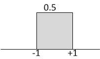
This can be done as follows\begin{align*} F\left ( \frac{1}{2}rect\left ( x\right ) \right ) & =\int _{-1}^{1}\frac{1}{2}e^{-i\omega x}dx=\frac{1}{2}\left ( \frac{e^{-i\omega x}}{-i\omega }\right ) _{-1}^{1}=\frac{1}{2}\left ( \frac{e^{-i\omega }}{-i\omega }-\frac{e^{i\omega }}{-i\omega }\right ) =\frac{1}{2}\frac{-1}{\omega }\left ( \frac{e^{-i\omega }-e^{i\omega }}{i}\right ) \\ & =\frac{1}{2}\frac{1}{\omega }\left ( \frac{e^{i\omega }-e^{-i\omega }}{i}\right ) \\ & =\frac{1}{2}\frac{1}{\omega }\left ( 2\sin \omega \right ) \\ & =\left ( \frac{\sin \omega }{\omega }\right ) \end{align*}
Therefore\[ \frac{\sin \omega }{\omega }\iff \frac{1}{2}rect\left ( x\right ) \] But \(rect\left ( x\right ) \) with height of \(\frac{1}{2}\)can be constructed from the difference of two unit step functions each of height \(\frac{1}{2}\)as shown below. Hence\[ \frac{1}{2}rect\left ( x\right ) =\frac{1}{2}H\left ( 1-x\right ) -\frac{1}{2}H\left ( -x-1\right ) \]
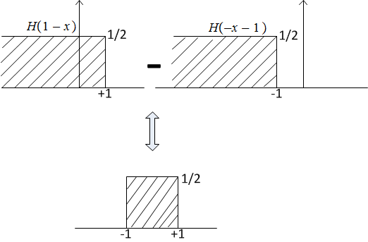
Therefore\begin{align*} \frac{\sin \omega }{\omega } & \iff \frac{1}{2}rect\left ( x\right ) \\ & \iff \frac{1}{2}\left ( H\left ( 1-x\right ) -H\left ( -x-1\right ) \right ) \end{align*}
Adding the frequency shifting from Eq. (2) gives the final result\begin{align*} \frac{\sin \left ( \omega -2\right ) }{\omega -2} & \iff e^{i2x}\mathcal{F}^{-1}\left ( \frac{\sin \omega }{\omega }\right ) \\ & \iff \frac{e^{i2x}}{2}\left ( \frac{1}{2}\left ( H\left ( 1-x\right ) -H\left ( -x-1\right ) \right ) \right ) \\ & =\frac{e^{i2x}}{4}\left ( H\left ( 1-x\right ) -H\left ( -x-1\right ) \right ) \end{align*}
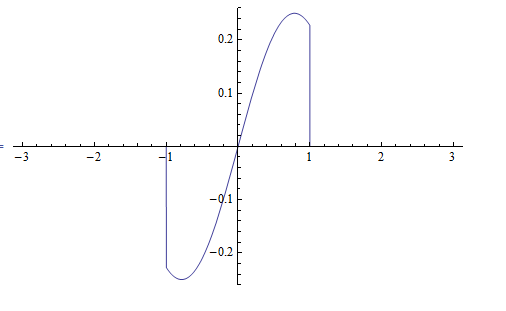
Or\[ \frac{\sin \left ( \omega -2\right ) }{\omega -2}\iff \frac{1}{4}\left ( \cos 2x+i\sin \left ( 2x\right ) \right ) \left ( H\left ( 1-x\right ) -H\left ( -x-1\right ) \right ) \] Here is a plot of the real part
Solve the integral equation \(\psi \left ( x\right ) =1+\lambda ^{2}\int _{0}^{x}\left ( t-x\right ) \) \(\psi \left ( t\right ) dt\)
solution
Taking derivative w.r.t. \(x\)\begin{align*} \psi ^{\prime }\left ( x\right ) & =\lambda ^{2}\left [ \int _{0}^{x}\frac{d}{dx}\left ( t-x\right ) \psi \left ( t\right ) dt+\frac{dx}{dx}\left ( \left ( t-x\right ) \psi \left ( t\right ) \right ) _{t=x}-0\right ] \\ & =\lambda ^{2}\left [ \int _{0}^{x}\frac{d}{dx}\left ( t\psi \left ( t\right ) -x\psi \left ( t\right ) \right ) dt+\overset{0}{\overbrace{\left ( \left ( x-x\right ) \psi \left ( x\right ) \right ) }}\right ] \\ & =-\lambda ^{2}\int _{0}^{x}\psi \left ( t\right ) dt \end{align*}
Taking another derivative\begin{align*} \psi ^{\prime \prime }\left ( x\right ) & =-\lambda ^{2}\left [ \int _{0}^{x}\frac{d}{dx}\psi \left ( t\right ) dt+\frac{dx}{dx}\left ( \psi \left ( t\right ) \right ) _{t=x}-0\right ] \\ & =-\lambda ^{2}\psi \left ( x\right ) \end{align*}
Hence\[ \psi ^{\prime \prime }\left ( x\right ) +\lambda ^{2}\psi \left ( x\right ) =0 \] The solution is \[ \psi \left ( x\right ) =A\cos \lambda x+B\sin \lambda x \] When \(x=0\) then \begin{align*} \psi \left ( 0\right ) & =1+\lambda ^{2}\int _{0}^{0}\left ( t-x\right ) \psi \left ( t\right ) dt\\ & =1 \end{align*}
Hence \begin{align*} A\cos \left ( \lambda 0\right ) +B\sin \left ( \lambda 0\right ) & =1\\ A & =1 \end{align*}
When \(x=0\) we also have \begin{align*} \psi ^{\prime }\left ( 0\right ) & =-\lambda ^{2}\int _{0}^{0}\psi \left ( t\right ) dt\\ & =0 \end{align*}
Hence\begin{align*} 0 & =-A\lambda \sin \lambda x+B\lambda \cos \lambda x\\ & =B\lambda \end{align*}
Hence \(B=0\) and therefore the final solution is\[ \psi \left ( x\right ) =\cos \left ( \lambda x\right ) \]
Solve the integral equation \(\frac{dy\left ( t\right ) }{dt}=1-\sin \left ( t\right ) -\int _{0}^{t}y\left ( \tau \right ) d\tau \) with IC \(y\left ( 0\right ) =0\)
Solution:
Taking derivative w.r.t. \(t\) gives\begin{align*} y^{\prime \prime }\left ( t\right ) & =-\cos \left ( t\right ) -\left [ \int _{0}^{t}\frac{d}{dt}y\left ( \tau \right ) d\tau +\frac{dt}{dt}y\left ( t\right ) -0\right ] \\ & =-\cos \left ( t\right ) -y\left ( t\right ) \end{align*}
Hence \[ y^{\prime \prime }\left ( t\right ) +y\left ( t\right ) =-\cos \left ( t\right ) \] Hence \(y_{h}\left ( t\right ) =A\cos t+B\sin t\) and for particular solution, since the homogeneous solution contains \(\cos \) then add \(t\) to each trial solution, hence let \[ y_{p}=c_{1}t\cos t+c_{2}t\sin t \] Therefore \begin{align*} y_{p}^{\prime } & =c_{1}\left ( \cos t-t\sin t\right ) +c_{2}\left ( \sin t+t\cos t\right ) \\ & =c_{1}\cos t-c_{1}t\sin t+c_{2}\sin t+c_{2}t\cos t\\ y_{p}^{\prime \prime } & =c_{1}\left ( -\sin t-\left ( \sin t+t\cos t\right ) \right ) +c_{2}\left ( \cos t+\left ( \cos t-t\sin t\right ) \right ) \\ & =-c_{1}\sin t-c_{1}\sin t-c_{1}t\cos t+c_{2}\cos t+c_{2}\cos t-c_{2}t\sin t \end{align*}
DE becomes\begin{align*} -c_{1}\sin t-c_{1}\sin t-c_{1}t\cos t+c_{2}\cos t+c_{2}\cos t-c_{2}t\sin t+\left ( c_{1}t\cos t+c_{2}t\sin t\right ) & =-\cos \left ( t\right ) \\ \cos t\left ( -c_{1}t+2c_{2}+c_{1}t\right ) +\sin t\left ( -2c_{1}-c_{2}t+c_{2}t\right ) & =-\cos \left ( t\right ) \\ \cos t\left ( 2c_{2}\right ) +\sin t\left ( -2c_{1}\right ) & =-\cos \left ( t\right ) \end{align*}
Hence \begin{align*} 2c_{2} & =-1\\ c_{2} & =\frac{-1}{2} \end{align*}
And\begin{align*} -2c_{1} & =0\\ c_{1} & =0 \end{align*}
Hence \[ y_{p}=\frac{-1}{2}t\sin t \] Hence the general solution is\[ y\left ( t\right ) =A\cos t+B\sin t-\frac{1}{2}t\sin t \] Since \(y\left ( 0\right ) =0\) then\[ 0=A \] And the solution becomes\[ y\left ( t\right ) =B\sin t-\frac{1}{2}t\sin t \] But \begin{align*} y^{\prime }\left ( t\right ) & =B\cos t-\frac{1}{2}\left ( \sin t+t\cos t\right ) \\ y^{\prime }\left ( 0\right ) & =B \end{align*}
But from the integral equation \(y^{\prime }\left ( 0\right ) =1-\sin \left ( 0\right ) -\int _{0}^{0}y\left ( \tau \right ) d\tau \) \(=1\)Hence \[ B=1 \] And the solution is\[ y\left ( t\right ) =\sin t-\frac{1}{2}t\sin t \]
Given the matrix equation \(\mathbf{x}^{\prime }=A\mathbf{x}+\mathbf{f}\,\ \)show that the particular solution integral is given by \(\mathbf{v}\left ( t\right ) =X\left ( t\right ) \int X^{-1}\left ( t\right ) \mathbf{f}\left ( t\right ) dt\) where \(X\left ( t\right ) \) is the fundamental matrix for the homogeneous equation
Solution
Will use \(\Omega \left ( t\right ) \) for the fundamental matrix and not \(X\left ( t\right ) \) since that is what we used before and in the text book, to make it less confusing. Hence the problem is to show that particular solution integral is given by \(\mathbf{v}\left ( t\right ) =\Omega \left ( t\right ) \int \Omega ^{-1}\left ( t\right ) \mathbf{f}\left ( t\right ) dt\) where \(\Omega \left ( t\right ) \) is the fundamental matrix for the homogeneous equation\begin{align*} \mathbf{x}^{\prime } & =A\mathbf{x}+\mathbf{f}\,\\ \mathbf{x}^{\prime }-A\mathbf{x} & =\mathbf{f}\, \end{align*}
The homogeneous solution is the solution to\[ \mathbf{x}_{h}^{\prime }-A\mathbf{x}_{h}=\mathbf{0}\,\, \] The homogeneous solution is given by \[ \mathbf{x}_{h}=\Omega \left ( t\right ) \mathbf{c}\] Where \(\Omega \left ( t\right ) \) is the fundamental matrix and \(\mathbf{c}\) is vector of the constants of integration. The
Now the particular solution \(\mathbf{v}_{p}\) is found using the variation of parameters method for systems of equations.\[ \mathbf{x}=\mathbf{x}_{h}+\mathbf{v}_{p}\] To find the particular solution, assume \begin{equation} \mathbf{v}_{p}=\Omega \mathbf{u} \tag{1} \end{equation} And \(\mathbf{u}\) is now found.\[ \mathbf{v}_{p}^{\prime }=\Omega ^{\prime }\mathbf{u+}\Omega \mathbf{u}^{\prime }\] Substituting the above in the original system ode \(\mathbf{x}^{\prime }=A\mathbf{x+f}\) gives\begin{align*} \mathbf{v}_{p}^{\prime } & =A\mathbf{v}_{p}\mathbf{+f}\\ \Omega ^{\prime }\mathbf{u}+\Omega \mathbf{u}^{\prime } & =\left ( A\Omega \right ) \mathbf{u+f} \end{align*}
But \(\Omega ^{\prime }=A\Omega \) (since \(\Omega \) is a fundamental solution, hence it satisfies the homogeneous DE) then the above simplifies to\begin{align*} \Omega ^{\prime }\mathbf{u}+\Omega \mathbf{u}^{\prime } & =\Omega ^{\prime }\mathbf{u+f}\\ \Omega \mathbf{u}^{\prime } & =\mathbf{f}\\ \mathbf{u}^{\prime } & =\Omega ^{-1}\mathbf{f}\\ \mathbf{u} & =\int \Omega ^{-1}\mathbf{f}\,\mathrm{d}t \end{align*}
Hence, Eq (1) becomes\[ \mathbf{v}\left ( t\right ) =\Omega \left ( t\right ) \int \Omega ^{-1}\left ( t\right ) \mathbf{f}\left ( t\right ) \,\mathrm{d}t \] Which is what we are asked to show.
Obtain solution to
\begin{align*} x^{\prime }+y^{\prime }+x & =-e^{-t}\\ x^{\prime }+2y^{\prime }+2x+2y & =0 \end{align*}
With IC \(x\left ( 0\right ) =-1,y\left ( 0\right ) =1\)
Solution:
The first step is to convert the system to \(\mathbf{x}^{\prime }=A\mathbf{x}+\mathbf{f}\,\) form. From first equation \(x^{\prime }=-y^{\prime }-x-e^{-t}\), substituting this in the second equation gives\[ -y^{\prime }-x-e^{-t}+2y^{\prime }+2x+2y=0 \] Solving for \(y^{\prime }\) gives\[ y^{\prime }=-x-2y+e^{-t}\] Substituting this in the first equation gives\begin{align*} x^{\prime }+e^{-t}-x-2y+x & =-e^{-t}\\ x^{\prime } & =-e^{-t}-e^{-t}+x+2y-x\\ & =2y-2e^{-t} \end{align*}
Therefore the system becomes\begin{align*} x^{\prime } & =2y-2e^{-t}\\ y^{\prime } & =-x-2y+e^{-t} \end{align*}
Or\[ \overset{\mathbf{x}^{\prime }}{\overbrace{\begin{pmatrix} x^{\prime }\\ y^{\prime }\end{pmatrix} }}=\overset{A}{\overbrace{\begin{pmatrix} 0 & 2\\ -1 & -2 \end{pmatrix} }}\overset{\mathbf{x}}{\overbrace{\begin{pmatrix} x\\ y \end{pmatrix} }}+\overset{\mathbf{f}}{\overbrace{\begin{pmatrix} -2\\ 1 \end{pmatrix} e^{-t}}}\] To find the eigenvalues of \(A\), the roots of the characteristic polynomial are found.\begin{align*} \left \vert A-\lambda I\right \vert & =0\\ \left \vert \begin{pmatrix} 0 & 2\\ -1 & -2 \end{pmatrix} -\begin{pmatrix} \lambda & 0\\ 0 & \lambda \end{pmatrix} \right \vert & =0\\ \left \vert \begin{pmatrix} -\lambda & 2\\ -1 & -2-\lambda \end{pmatrix} \right \vert & =0\\ \left ( -\lambda \right ) \left ( -2-\lambda \right ) +2 & =0\\ \lambda ^{2}+2\lambda +2 & =0 \end{align*}
The roots are \(\frac{-b\pm \sqrt{b^{2}-4ac}}{2a}=\frac{-2\pm \sqrt{4-8}}{2}=\frac{-2\pm \sqrt{-4}}{2}=\frac{-2\pm 2i}{2}=-1\pm i\), hence eigenvalues are \[ \left \{ -1-i,-1+i\right \} \] To find the eigenvectors\begin{align*} \left ( A-I\lambda \right ) \mathbf{v}_{1} & =0\\\begin{pmatrix} -\lambda & 2\\ -1 & -2-\lambda \end{pmatrix}\begin{pmatrix} v_{11}\\ v_{21}\end{pmatrix} & =\begin{pmatrix} 0\\ 0 \end{pmatrix} \end{align*}
For \(\lambda _{1}=-1-i\), hence\begin{align*} \begin{pmatrix} -\left ( -1-i\right ) & 2\\ -1 & -2-\left ( -1-i\right ) \end{pmatrix}\begin{pmatrix} v_{11}\\ v_{21}\end{pmatrix} & =\begin{pmatrix} 0\\ 0 \end{pmatrix} \\\begin{pmatrix} 1+i & 2\\ -1 & -1+i \end{pmatrix}\begin{pmatrix} v_{11}\\ v_{21}\end{pmatrix} & =\begin{pmatrix} 0\\ 0 \end{pmatrix} \\\begin{pmatrix} \left ( 1+i\right ) v_{11}+2v_{21}\\ -v_{11}+\left ( -1+i\right ) v_{21}\end{pmatrix} & =\begin{pmatrix} 0\\ 0 \end{pmatrix} \end{align*}
Let \(v_{21}=1\), and find \(v_{11}\), hence from first equation \(\left ( 1+i\right ) v_{11}+2=0\) then \(v_{11}=\frac{-2}{1+i}=\frac{-2\left ( 1-i\right ) }{\left ( 1+i\right ) \left ( 1-i\right ) }=\frac{-2+2i}{1+1}=-1+i\)
Hence the first eigenvector is\[ \mathbf{v}_{1}=\begin{pmatrix} -1+i\\ 1 \end{pmatrix} \] For \(\lambda _{1}=-1+i\),\begin{align*} \begin{pmatrix} -\left ( -1+i\right ) & 2\\ -1 & -2-\left ( -1+i\right ) \end{pmatrix}\begin{pmatrix} v_{12}\\ v_{22}\end{pmatrix} & =\begin{pmatrix} 0\\ 0 \end{pmatrix} \\\begin{pmatrix} 1-i & 2\\ -1 & -1-i \end{pmatrix}\begin{pmatrix} v_{12}\\ v_{22}\end{pmatrix} & =\begin{pmatrix} 0\\ 0 \end{pmatrix} \\\begin{pmatrix} \left ( 1-i\right ) v_{12}+2v_{22}\\ -v_{12}+\left ( -1-i\right ) v_{21}\end{pmatrix} & =\begin{pmatrix} 0\\ 0 \end{pmatrix} \end{align*}
Let \(v_{22}=1\), and find \(v_{12}\), hence from first equation \(\left ( 1-i\right ) v_{12}+2=0\) then \(v_{12}=\frac{-2}{1-i}=\frac{-2\left ( 1+i\right ) }{\left ( 1-i\right ) \left ( 1+i\right ) }=\frac{-2-2i}{1+1}=-1-i\)
Hence the second eigenvector is\[ \mathbf{v}_{2}=\begin{pmatrix} -1-i\\ 1 \end{pmatrix} \] Therefore, the matrix of eigenvectors is\begin{align*} P & =\begin{pmatrix} \mathbf{v}_{1} & \mathbf{v}_{2}\end{pmatrix} \\ & =\begin{pmatrix} -1+i & -1-i\\ 1 & 1 \end{pmatrix} \end{align*}
And the matrix of eigenvalues is\[ D=\begin{pmatrix} -1-i & 0\\ 0 & -1+i \end{pmatrix} \] Hence the fundamental matrix is\[ \Omega =\begin{pmatrix} \left ( -1+i\right ) e^{\left ( -1-i\right ) t} & \left ( -1-i\right ) e^{\left ( -1+i\right ) t}\\ e^{\left ( -1-i\right ) t} & e^{\left ( -1+i\right ) t}\end{pmatrix} \] Now the system is decoupled in order to solve it. Let \(\mathbf{x}=P\mathbf{z}\) hence \(\mathbf{x}^{\prime }=A\mathbf{x}+\mathbf{f}\,\) becomes\[ P\mathbf{z}^{\prime }=AP\mathbf{z}+f \] Premultiply by \(P^{-1}\) simplifies to (since \(P^{-1}P=I)\)\begin{align*} \mathbf{z}^{\prime } & =P^{-1}AP\mathbf{z}+P^{-1}\mathbf{f}\\ & =D\mathbf{z}+\mathbf{G} \end{align*}
Where \[ \mathbf{G=}P^{-1}\mathbf{f=}\begin{pmatrix} -1+i & -1-i\\ 1 & 1 \end{pmatrix} ^{-1}\begin{pmatrix} -2\\ 1 \end{pmatrix} e^{-t}\] But \(\begin{pmatrix} -1+i & -1-i\\ 1 & 1 \end{pmatrix} ^{-1}=\frac{1}{2}\) \(\begin{pmatrix} -i & 1-i\\ i & 1+i \end{pmatrix} \), so \begin{align*} \mathbf{G} & \mathbf{=}\frac{1}{2}\begin{pmatrix} -i & 1-i\\ i & 1+i \end{pmatrix}\begin{pmatrix} -2\\ 1 \end{pmatrix} e^{-t}\\ & =\frac{1}{2}\begin{pmatrix} 1+i\\ 1-i \end{pmatrix} e^{-t} \end{align*}
The above system is decoupled since \(D\) is diagonal\begin{align*} \begin{pmatrix} z_{1}^{\prime }\\ z_{2}^{\prime }\end{pmatrix} & =\begin{pmatrix} -1-i & 0\\ 0 & -1+i \end{pmatrix}\begin{pmatrix} z_{1}\\ z_{2}\end{pmatrix} +\mathbf{G}\\ & =\begin{pmatrix} -1-i & 0\\ 0 & -1+i \end{pmatrix}\begin{pmatrix} z_{1}\\ z_{2}\end{pmatrix} +\frac{1}{2}\begin{pmatrix} 1+i\\ 1-i \end{pmatrix} e^{-t}\\ & =\begin{pmatrix} \left ( -1-i\right ) z_{1}+\frac{1}{2}\left ( 1+i\right ) e^{-t}\\ \left ( -1+i\right ) z_{2}+\frac{1}{2}\left ( 1-i\right ) e^{-t}\end{pmatrix} \end{align*}
Hence \begin{align*} z_{1}^{\prime }\left ( t\right ) & =\left ( -1-i\right ) z_{1}\left ( t\right ) +\frac{1}{2}\left ( 1+i\right ) e^{-t}\\ z_{2}^{\prime }\left ( t\right ) & =\left ( -1+i\right ) z_{2}\left ( t\right ) +\frac{1}{2}\left ( 1-i\right ) e^{-t} \end{align*}
The first equation gives\[ z_{1}^{\prime }\left ( t\right ) +\left ( 1+i\right ) z_{1}\left ( t\right ) =\frac{1}{2}\left ( 1+i\right ) e^{-t}\] The integrating factor is \(e^{\int \left ( 1+i\right ) dt}=e^{\left ( 1+i\right ) t}\), hence the solution is\begin{align*} d\left ( e^{\left ( 1+i\right ) t}z_{1}\left ( t\right ) \right ) & =e^{\left ( 1+i\right ) t}\frac{1}{2}\left ( 1+i\right ) e^{-t}\\ e^{\left ( 1+i\right ) t}z_{1}\left ( t\right ) & =\int e^{\left ( 1+i\right ) t}\frac{1}{2}\left ( 1+i\right ) e^{-t}dt+C_{1}\\ z_{1}\left ( t\right ) & =e^{-\left ( 1+i\right ) t}\int e^{\left ( 1+i\right ) t}\frac{1}{2}\left ( 1+i\right ) e^{-t}dt+e^{-\left ( 1+i\right ) t}C_{1}\\ & =\frac{1}{2}e^{-\left ( 1+i\right ) t}\int e^{it}\left ( 1+i\right ) dt+e^{-\left ( 1+i\right ) t}C_{1}\\ & =\frac{1}{2}e^{-\left ( 1+i\right ) t}\int \left ( e^{it}+ie^{it}\right ) dt+e^{-\left ( 1+i\right ) t}C_{1}\\ & =\frac{1}{2}e^{-t}e^{-it}\left ( \frac{e^{it}}{i}+i\frac{e^{it}}{i}\right ) +e^{-\left ( 1+i\right ) t}C_{1}\\ & =\frac{1}{2}e^{-t}e^{-it}\left ( -ie^{it}+e^{it}\right ) +e^{-\left ( 1+i\right ) t}C_{1}\\ & =\frac{1}{2}e^{-t}\left ( -i+1\right ) +e^{-\left ( 1+i\right ) t}C_{1}\\ & =-\frac{1}{2}ie^{-t}+\frac{1}{2}e^{-t}+e^{-\left ( 1+i\right ) t}C_{1} \end{align*}
And\begin{align*} z_{2}^{\prime }\left ( t\right ) & =\left ( -1+i\right ) z_{2}\left ( t\right ) +\frac{1}{2}\left ( 1-i\right ) e^{-t}\\ z_{2}^{\prime }\left ( t\right ) +\left ( 1-i\right ) z_{2}\left ( t\right ) & =\frac{1}{2}\left ( 1-i\right ) e^{-t} \end{align*}
The integrating factor is \(e^{\int \left ( 1-i\right ) dt}=e^{\left ( 1-i\right ) t}\), hence the solution is\begin{align*} d\left ( e^{\left ( 1-i\right ) t}z_{2}\left ( t\right ) \right ) & =e^{\left ( 1-i\right ) t}\frac{1}{2}\left ( 1-i\right ) e^{-t}\\ e^{\left ( 1-i\right ) t}z_{2}\left ( t\right ) & =\int e^{\left ( 1-i\right ) t}\frac{1}{2}\left ( 1-i\right ) e^{-t}dt+C_{2}\\ z_{2}\left ( t\right ) & =e^{-\left ( 1-i\right ) t}\int e^{\left ( 1-i\right ) t}\frac{1}{2}\left ( 1-i\right ) e^{-t}dt+e^{-\left ( 1-i\right ) t}C_{2}\\ & =\frac{1}{2}e^{-\left ( 1-i\right ) t}\int e^{-it}\left ( 1-i\right ) dt+e^{-\left ( 1-i\right ) t}C_{2}\\ & =\frac{1}{2}e^{-\left ( 1-i\right ) t}\int \left ( e^{-it}-ie^{-it}\right ) dt+e^{-\left ( 1-i\right ) t}C_{2}\\ & =\frac{1}{2}e^{-t}e^{it}\left ( \frac{e^{-it}}{-i}-i\frac{e^{-it}}{-i}\right ) +e^{-\left ( 1-i\right ) t}C_{2}\\ & =\frac{1}{2}e^{-t}e^{it}\left ( ie^{-it}+e^{-it}\right ) +e^{-\left ( 1-i\right ) t}C_{2}\\ & =\frac{1}{2}e^{-t}\left ( i+1\right ) +e^{-\left ( 1-i\right ) t}C_{2}\\ & =\frac{1}{2}ie^{-t}+\frac{1}{2}e^{-t}+e^{-\left ( 1-i\right ) t}C_{2} \end{align*}
Hence\[\begin{pmatrix} z_{1}\left ( t\right ) \\ z_{2}\left ( t\right ) \end{pmatrix} =\begin{pmatrix} -\frac{1}{2}ie^{-t}+\frac{1}{2}e^{-t}+e^{-\left ( 1+i\right ) t}C_{1}\\ \frac{1}{2}ie^{-t}+\frac{1}{2}e^{-t}+e^{-\left ( 1-i\right ) t}C_{2}\end{pmatrix} \] And since \(\mathbf{x}=P\mathbf{z}\) then\begin{align*} \begin{pmatrix} x\left ( t\right ) \\ y\left ( t\right ) \end{pmatrix} & =\begin{pmatrix} -1+i & -1-i\\ 1 & 1 \end{pmatrix}\begin{pmatrix} -\frac{1}{2}ie^{-t}+\frac{1}{2}e^{-t}+e^{-\left ( 1+i\right ) t}C_{1}\\ \frac{1}{2}ie^{-t}+\frac{1}{2}e^{-t}+e^{-\left ( 1-i\right ) t}C_{2}\end{pmatrix} \\ & =\begin{pmatrix} \left ( -1+i\right ) \left ( -\frac{1}{2}ie^{-t}+\frac{1}{2}e^{-t}+e^{-\left ( 1+i\right ) t}C_{1}\right ) +\left ( -1-i\right ) \frac{1}{2}ie^{-t}+\frac{1}{2}e^{-t}+e^{-\left ( 1-i\right ) t}C_{2}\\ \left ( -\frac{1}{2}ie^{-t}+\frac{1}{2}e^{-t}+e^{-\left ( 1+i\right ) t}C_{1}\right ) +\frac{1}{2}ie^{-t}+\frac{1}{2}e^{-t}+e^{-\left ( 1-i\right ) t}C_{2}\end{pmatrix} \\ & =\begin{pmatrix} \left ( 1+\frac{1}{2}i\right ) e^{-t}-\left ( 1-i\right ) C_{1}e^{-\left ( 1+i\right ) t}+C_{2}e^{-\left ( 1-i\right ) t}\\ e^{-t}+C_{1}e^{-\left ( 1+i\right ) t}+C_{2}e^{-\left ( 1-i\right ) t}\end{pmatrix} \\ & =\begin{pmatrix} e^{-t}+\frac{1}{2}ie^{-t}-\left ( 1-i\right ) C_{1}e^{-t}e^{-it}+C_{2}e^{-t}e^{it}\\ e^{-t}+C_{1}e^{-t}e^{-it}+C_{2}e^{-t}e^{it}\end{pmatrix} \\ & =\begin{pmatrix} e^{-t}+\frac{1}{2}ie^{-t}-C_{1}e^{-t}e^{-it}+iC_{1}e^{-t}e^{-it}+C_{2}e^{-t}e^{it}\\ e^{-t}+C_{1}e^{-t}e^{-it}+C_{2}e^{-t}e^{it}\end{pmatrix} \end{align*}
The above can be simplified more if needed using Euler relation.\begin{align*} x\left ( t\right ) & =e^{-t}+\frac{1}{2}ie^{-t}-C_{1}e^{-t}e^{-it}+iC_{1}e^{-t}e^{-it}+C_{2}e^{-t}e^{it}\\ y\left ( t\right ) & =e^{-t}+C_{1}e^{-t}e^{-it}+C_{2}e^{-t}e^{it} \end{align*}
\(C_{1},C_{2}\) can be found from I.C.

Solution
Using the following relations for \(0<t<\infty \), where \(\mathcal{F}\left ( f\left ( t\right ) \right ) \equiv F\left ( \omega \right ) \)\begin{align*} \mathcal{F}\left ( f^{\prime }\left ( t\right ) \right ) & =i\omega F\left ( \omega \right ) -f\left ( 0\right ) \\\mathcal{F}\left ( f^{\prime \prime }\left ( t\right ) \right ) & =\left ( i\omega \right ) ^{2}F\left ( \omega \right ) -i\omega f\left ( 0\right ) -f^{\prime }\left ( 0\right ) \end{align*}
Now we need to take the Fourier transform of \(3y^{\prime \prime }\left ( t\right ) +10y^{\prime }\left ( t\right ) +3y\left ( t\right ) =64e^{3t}\left ( H\left ( t\right ) -H\left ( t-5\right ) \right ) \). The first step is to normalize the leading term, this will make it easier later. Hence the ODE becomes\[ y^{\prime \prime }\left ( t\right ) +\frac{10}{3}y^{\prime }\left ( t\right ) +y\left ( t\right ) =\frac{64}{3}e^{3t}\left ( H\left ( t\right ) -H\left ( t-5\right ) \right ) \] But\begin{align*} \mathcal{F}\left ( \frac{64}{3}e^{3t}\left ( H\left ( t\right ) -H\left ( t-5\right ) \right ) \right ) & =\frac{64}{3}\int _{0}^{5}e^{3t}e^{-i\omega t}dt\\ & =\frac{64}{3}\int _{0}^{5}e^{-t(i\omega -3)}dt\\ & =\frac{64}{3}\left [ \frac{e^{-t(i\omega -3)}}{-\left ( i\omega -3\right ) }\right ] _{0}^{5}=\frac{64}{3}\frac{e^{-5(i\omega -3)}-1}{-\left ( i\omega -3\right ) } \end{align*}
Hence the Fourier transform of the ODE becomes\[ \left ( \left ( i\omega \right ) ^{2}F\left ( \omega \right ) -i\omega f\left ( 0\right ) -f^{\prime }\left ( 0\right ) \right ) +\frac{10}{3}\left ( i\omega F\left ( \omega \right ) -f\left ( 0\right ) \right ) +F\left ( \omega \right ) =\frac{64}{3}\frac{e^{-5(i\omega -3)}}{-\left ( i\omega -3\right ) }+\frac{64}{3}\frac{1}{\left ( i\omega -3\right ) }\] Applying initial conditions\begin{align*} \left ( -\omega ^{2}F\left ( \omega \right ) +i\omega \right ) +\frac{10}{3}\left ( i\omega F\left ( \omega \right ) +1\right ) +F\left ( \omega \right ) & =\frac{64}{3}\frac{e^{-5(i\omega -3)}}{-\left ( i\omega -3\right ) }+\frac{64}{3}\frac{1}{\left ( i\omega -3\right ) }\\ -\omega ^{2}F\left ( \omega \right ) +i\omega +\frac{10}{3}i\omega F\left ( \omega \right ) +\frac{10}{3}+F\left ( \omega \right ) & =\frac{64}{3}\frac{e^{-5(i\omega -3)}}{-\left ( i\omega -3\right ) }+\frac{64}{3}\frac{1}{\left ( i\omega -3\right ) }\\ F\left ( \omega \right ) \left ( -\omega ^{2}+\frac{10}{3}i\omega +1\right ) & =\frac{64}{3}\frac{e^{-5(i\omega -3)}}{-\left ( i\omega -3\right ) }+\frac{64}{3}\frac{1}{\left ( i\omega -3\right ) }-i\omega -\frac{10}{3}\\ F\left ( \omega \right ) \left ( \omega ^{2}-\frac{10}{3}i\omega -1\right ) & =\frac{64}{3}\frac{e^{-5(i\omega -3)}}{\left ( i\omega -3\right ) }-\frac{64}{3}\frac{1}{\left ( i\omega -3\right ) }+i\omega +\frac{10}{3} \end{align*}
Solving for \(F\left ( \omega \right ) \)\begin{align*} F\left ( \omega \right ) & =\frac{64}{3}\frac{e^{-5(i\omega -3)}}{\left ( i\omega -3\right ) \left ( \omega ^{2}-\frac{10}{3}i\omega -1\right ) }-\frac{64}{3}\frac{1}{\left ( i\omega -3\right ) \left ( \omega ^{2}-\frac{10}{3}i\omega -1\right ) }\\ & +\frac{i\omega }{\left ( \omega ^{2}-\frac{10}{3}i\omega -1\right ) }+\frac{10}{3\left ( \omega ^{2}-\frac{10}{3}i\omega -1\right ) } \end{align*}
But \(\left ( \omega ^{2}-\frac{10}{3}i\omega -1\right ) =\allowbreak \left ( \omega -\frac{1}{3}i\right ) \left ( \omega -3i\right ) \) hence the above becomes\begin{align*} F\left ( \omega \right ) & =\frac{64e^{15}}{3}\frac{e^{-5i\omega }}{\left ( i\omega -3\right ) \left ( \omega -\frac{1}{3}i\right ) \left ( \omega -3i\right ) }-\frac{64}{3}\frac{1}{\left ( i\omega -3\right ) \left ( \omega -\frac{1}{3}i\right ) \left ( \omega -3i\right ) }\\ & +\frac{i\omega }{\left ( \omega -\frac{1}{3}i\right ) \left ( \omega -3i\right ) }+\frac{10}{3}\frac{1}{\left ( \omega -\frac{1}{3}i\right ) \left ( \omega -3i\right ) } \end{align*}
We now start to do inverse Fourier transform\(.\) For the first integral, using the Fourier shift in time property \[ e^{-i5\omega }F\left ( \omega \right ) \iff f\left ( t-5\right ) \] Hence we just need to find \(f\left ( t\right ) \) for the first term and then shift it in time. The first term now becomes\[ T_{1}=\frac{1}{\left ( i\omega -3\right ) \left ( \omega -\frac{1}{3}i\right ) \left ( \omega -3i\right ) }\] Partial fractions give\[ T_{1}=\frac{1}{16}\frac{i}{\omega -3i}+\frac{1}{20}\frac{i}{\omega +3i}-\frac{9}{80}\frac{i}{\omega -\frac{1}{3}i}\] Using property \(\mathcal{F}^{-1}\left ( \frac{1}{i\omega +a}\right ) =e^{-at}H\left ( t\right ) \) and \(\mathcal{F}^{-1}\left ( \frac{1}{i\omega -a}\right ) =-e^{at}H\left ( -t\right ) \) \begin{align*} \frac{1}{16}\mathcal{F}^{-1}\left ( \frac{i}{\omega -3i}\right ) & =\frac{1}{16}\mathcal{F}^{-1}\left ( \frac{-1}{\omega i+3}\right ) =-\frac{1}{16}e^{-3t}H\left ( t\right ) \\ \frac{1}{20}\mathcal{F}^{-1}\left ( \frac{i}{\omega +3i}\right ) & =\frac{1}{20}\mathcal{F}^{-1}\left ( \frac{-1}{\omega i-3}\right ) =-\frac{1}{20}e^{3t}H\left ( -t\right ) \\ -\frac{9}{80}\mathcal{F}^{-1}\left ( \frac{i}{\omega -\frac{1}{3}i}\right ) & =-\frac{9}{80}\mathcal{F}^{-1}\left ( \frac{-1}{\omega i+\frac{1}{3}}\right ) =+\frac{9}{80}e^{-\frac{t}{3}}H\left ( t\right ) \end{align*}
Terms with \(H\left ( -t\right ) \) do not count, since these are only defined for negative time. The solution is only valid for \(t>0\), therefore these terms are ignored in the final solution. Hence \begin{align*} \mathcal{F}^{-1}\left ( \frac{64e^{15}}{3}\frac{e^{-5i\omega }}{\left ( i\omega -3\right ) \left ( \omega -\frac{1}{3}i\right ) \left ( \omega -3i\right ) }\right ) & =\frac{64e^{15}}{3}\left ( -\frac{1}{16}e^{-3t}H\left ( t\right ) +\frac{9}{80}e^{-\frac{t}{3}}H\left ( t\right ) \right ) _{t=t-5}\\ & =\frac{64e^{15}}{3}\left ( -\frac{1}{16}e^{-3\left ( t-5\right ) }H\left ( t-5\right ) +\frac{9}{80}e^{-\frac{t-5}{3}}H\left ( t-5\right ) \right ) \end{align*}
Ok, one term is done. Four more to go. Looking at \(T_{2}=-\frac{64}{3}\frac{1}{\left ( i\omega -3\right ) \left ( \omega -\frac{1}{3}i\right ) \left ( \omega -3i\right ) }\) this is the same as above, but with no time shift, hence\[\mathcal{F}^{-1}\left ( -\frac{64}{3}\frac{1}{\left ( i\omega -3\right ) \left ( \omega -\frac{1}{3}i\right ) \left ( \omega -3i\right ) }\right ) =\frac{64}{3}\left ( -\frac{1}{16}e^{-3t}H\left ( t\right ) +\frac{9}{80}e^{-\frac{t}{3}}H\left ( t\right ) \right ) \] Looking at \(T_{3}=\frac{i\omega }{\left ( \omega -\frac{1}{3}i\right ) \left ( \omega -3i\right ) }\) partial fractions gives \(T_{2}\allowbreak =\frac{9}{8}\frac{i}{\omega -3i}-\frac{1}{8}\frac{i}{\omega -\frac{1}{3}i}\) hence\[\mathcal{F}^{-1}\left ( \frac{9}{8}\frac{i}{\omega -3i}-\frac{1}{8}\frac{i}{\omega -\frac{1}{3}i}\right ) =\frac{-9}{8}e^{-3t}H\left ( t\right ) +\frac{1}{8}e^{-\frac{t}{3}}H\left ( t\right ) \] And finally, \(T_{4}=\frac{10}{3}\frac{1}{\left ( \omega -\frac{1}{3}i\right ) \left ( \omega -3i\right ) }\) and partial fractions gives \(T_{4}=\frac{10}{3}\left ( \frac{3}{8}\frac{i}{\omega -\frac{1}{3}i}-\frac{3}{8}\frac{i}{\omega -3i}\right ) \), hence\[\mathcal{F}^{-1}\left ( \frac{10}{8}\frac{i}{\omega -\frac{1}{3}i}-\frac{10}{8}\frac{i}{\omega -3i}\right ) =\frac{-10}{8}e^{-\frac{t}{3}}H\left ( t\right ) +\frac{10}{8}e^{-3t}H\left ( t\right ) \] Collecting all terms, the final result is\begin{align*} y\left ( t\right ) & =\frac{64e^{15}}{3}\left ( -\frac{1}{16}e^{-3\left ( t-5\right ) }H\left ( t-5\right ) +\frac{9}{80}e^{-\frac{t-5}{3}}H\left ( t-5\right ) \right ) \\ & +\frac{64}{3}\left ( -\frac{1}{16}e^{-3t}H\left ( t\right ) +\frac{9}{80}e^{-\frac{t}{3}}H\left ( t\right ) \right ) \\ & \frac{-9}{8}e^{-3t}H\left ( t\right ) +\frac{1}{8}e^{-\frac{t}{3}}H\left ( t\right ) \\ & \frac{-10}{8}e^{-\frac{t}{3}}H\left ( t\right ) +\frac{10}{8}e^{-3t}H\left ( t\right ) \end{align*}
Expanding and collecting\begin{align*} y\left ( t\right ) & =\frac{64e^{15}}{3}H\left ( t-5\right ) \left ( -\frac{1}{16}e^{-3\left ( t-5\right ) }+\frac{9}{80}e^{-\frac{t-5}{3}}\right ) \\ & +H\left ( t\right ) \left ( -\frac{1}{16}e^{-3t}+\frac{9}{80}e^{-\frac{t}{3}}-\frac{9}{8}e^{-3t}+\frac{1}{8}e^{-\frac{t}{3}}-\frac{10}{8}e^{-\frac{t}{3}}+\frac{10}{8}e^{-3t}\right ) \\ & \\ & =\frac{64e^{15}}{3}H\left ( t-5\right ) \left ( -\frac{1}{16}e^{-3\left ( t-5\right ) }+\frac{9}{80}e^{-\frac{t-5}{3}}\right ) \\ & +H\left ( t\right ) \left ( \frac{1}{16}e^{-3t}-\frac{81}{80}e^{-\frac{1}{3}t}\right ) \end{align*}
Therefore the solution is\[ y\left ( t\right ) =\left \{ \begin{array} [c]{ccc}\frac{64e^{15}}{3}\left ( -\frac{1}{16}e^{-3\left ( t-5\right ) }+\frac{9}{80}e^{-\frac{t-5}{3}}\right ) +\left ( \frac{1}{16}e^{-3t}-\frac{81}{80}e^{-\frac{1}{3}t}\right ) & & 0<t\leq 5\\ \frac{1}{16}e^{-3t}-\frac{81}{80}e^{-\frac{1}{3}t} & & 5<t<\infty \end{array} \right . \]