
Matlab was used to generate the contour plots. The plots generated are given below and the source code used is listed in the appendix.

Matlab 2015a was used to implement steepest descent algorithm. Listing is given in the appendix. The following is the outline of general algorithm expressed as pseudo code.

In all of the following results, the convergence to optimal was determined as follows: First a maximum number of iterations was used to guard against slow convergence or other unforeseen cases. This is a safety measure. It is always recommended to use in any iterative method. This number was set very high at one million iterations. If convergence was not reached by this count, the iterations stop.
The second check was the main criteria, which is to check that the norm of the gradient \(\left | \nabla (J(u)) \right | \) has reached a minimum value. Since \(\left | \nabla (J(u)) \right | \) is zero at the optimal point, this check is the most common one to use to stop the iterations. The norm was calculated after each step. When \(\left | \nabla (J(u)) \right | \) became smaller than \(0.01\), the search stopped. The value \(0.01\) was selected arbitrarily. All cases below used the same convergence criterion.
A third check was added to verify that the value of the objective function \(J(u)\) did not increase after each step. If \(J(u)\) increased the search stops, as this indicates the step size taken is too large and oscillation has started. This condition happened many times when using fixed step size, but it did not happen with optimal step size.
The relevant Matlab code used to implement this convergence criteria is the following:
The result of these runs are given below in table form. For each starting point, the search path \(u^k\) is plotted on top of the contour plot. Animation of each of these is also available when running the code. The path \(u^k\) shows that search direction is along the gradient vector, which is perpendicular to the tangent line at each contour level.


When trying different values of starting points, all with \(u_{1}>1,u_{2}>0\), the search did converge to \(u^{\ast }=[7,-2]\), but it also depended on where the search started from. When starting close to \(u^{\ast }\), for example, from \(u^0=[6.5,1]\) the search did converge using fixed step size of \(h=0.01\) with no oscillation seen. Below shows this result

However, when starting from a point too far away from \((7,-2)\), it did not converge to \((7,-2)\), but instead converged to the second local minimum at \(u^{\ast }=[13,4]\) as seen below. In this case the search started from \([20,20]\).
If the starting point was relatively close to one local minimum than the other, the search will converge to nearest local minimum.

In this problem there are two local minimums, one at \((7,-2)\) and the other at \((4,13)\). It depends on the location of the starting point \(u^0\) as to which \(u^{\ast }\) the algorithm will converge to.


The steepest descent algorithm used in the first problem was modified to support an optimal step size. The following is the updated general algorithm expressed as pseudo code. The optimal step line search used was the standard golden section method. (Listing added to appendix).

For \(n=2\), the Rosenbrock function is \begin{align*} J(u) & = 100 \left ( u_2-u_{1}^{2}\right )^{2} + \left (1-u_{1}\right ) ^{2}\\ \nabla J\left ( u\right ) & =\begin{bmatrix} \frac{\partial J}{\partial u_{1}}\\ \frac{\partial J}{\partial u_{2}}\end{bmatrix} =\begin{bmatrix} -400\left ( u_{2}-u_{1}^{2}\right ) u_{1}-2\left ( 1-u_{1}\right ) \\ 200\left ( u_{2}-u_{1}^{2}\right ) \end{bmatrix} \end{align*}
For \[ -2.5\leq u_{i} \leq 2.5 \]
The steepest algorithm was run on the above function. The following is the contour plot. These plots show the level set by repeated zooming around at \((1,1)\), which is the location of the optimal point. The optimal value is at \(u^{\ast }=(1,1)\) where \(J^{\ast }=0\).


In all of the results below, where fixed step is compared to optimal step, the convergence criteria was the same. It was to stop the search when \[ \| \nabla J(u) \| \leq 0.001 \] The search started from different locations. The first observation was that when using optimal step, the search jumps very quickly into the small valley of the function moving towards \(u^{\ast }\). This used one or two steps only. After getting close to the optimal point, the search became very slow moving towards \(u^{\ast }\) inside the valley because the optimal step size was becoming smaller and smaller.
The closer the search was to \(u^{\ast }\), the step size became smaller. Convergence was very slow at the end. The plot below shows the optimal step size used each time. Zooming in shows the zigzag pattern. This pattern was more clear when using small but fixed step size. Below is an example using fixed step size of \(h=0.01\) showing the pattern inside the valley of the function.

Here is a partial list of the level set values, starting from arbitrary point from one run using optimal step. It shows that in one step, \(J(u)\) went down from \(170\) to \(0.00038\), but after that the search became very slow and the optimal step size became smaller and the rate of reduction of \(J(u)\) decreased.
Golden section line search was implemented with tolerance of \(\sqrt (eps(\text{double}))\) and used for finding the optimal step size.
The following plot shows how the optimal step size changed at each iteration in a typical part of the search, showing how the step size becomes smaller and smaller as the search approaches the optimal point \(u^{\ast }\). The plot to the right shows the path \(u^k\) taken.


To compare fixed size step and optimal size \(h\), the search was started from the same point and the number of steps needed to converge was recorded.
In these runs, a maximum iteration limit was set at \(10^6\).
Starting from \((-2,0.8)\)
| step size |
number of iterations to converge |
| optimal |
4089 |
| \(0.1\) |
Did not converge within maximum iteration limit |
| \(0.05\) | Did not converge within maximum iteration limit, but stopped closer to \(u^{\ast }\) than the above case using \(h=0.1\) |
| \(0.01\) |
Did not converge within maximum iteration limit, but stopped closer to \(u^{\ast }\) than the above case using \(h=0.05\) |
The following shows the path used in the above tests. The plots show that using fixed size step leads to many zigzag steps being taken which slows the search and is not efficient as using optimal step size.
Using fixed size \(h=0.1\) resulted in the search not making progress after some point due to oscillation and would be stuck in the middle of the valley.
Following is partial list of the values of \(J(u)\) at each iteration using fixed size \(h\), showing that the search fluctuating between two levels as it gets closer to optimal value \(u^{\ast }\) but it was not converging.
Search was terminated when oscillation is detected. Search stopped far away from \(u^{\ast }\) when the fixed step was large. As the fixed step size decreased, the final \(u^{k}\) that was reached was closer to \(u^{\ast }\) but did not converge to it within the maximum iteration limit as the case with optimal step size.
The optimal step size produced the best result. It converged to \(u^{\ast }\) within the maximum iteration limit and the zigzag pattern was smaller.


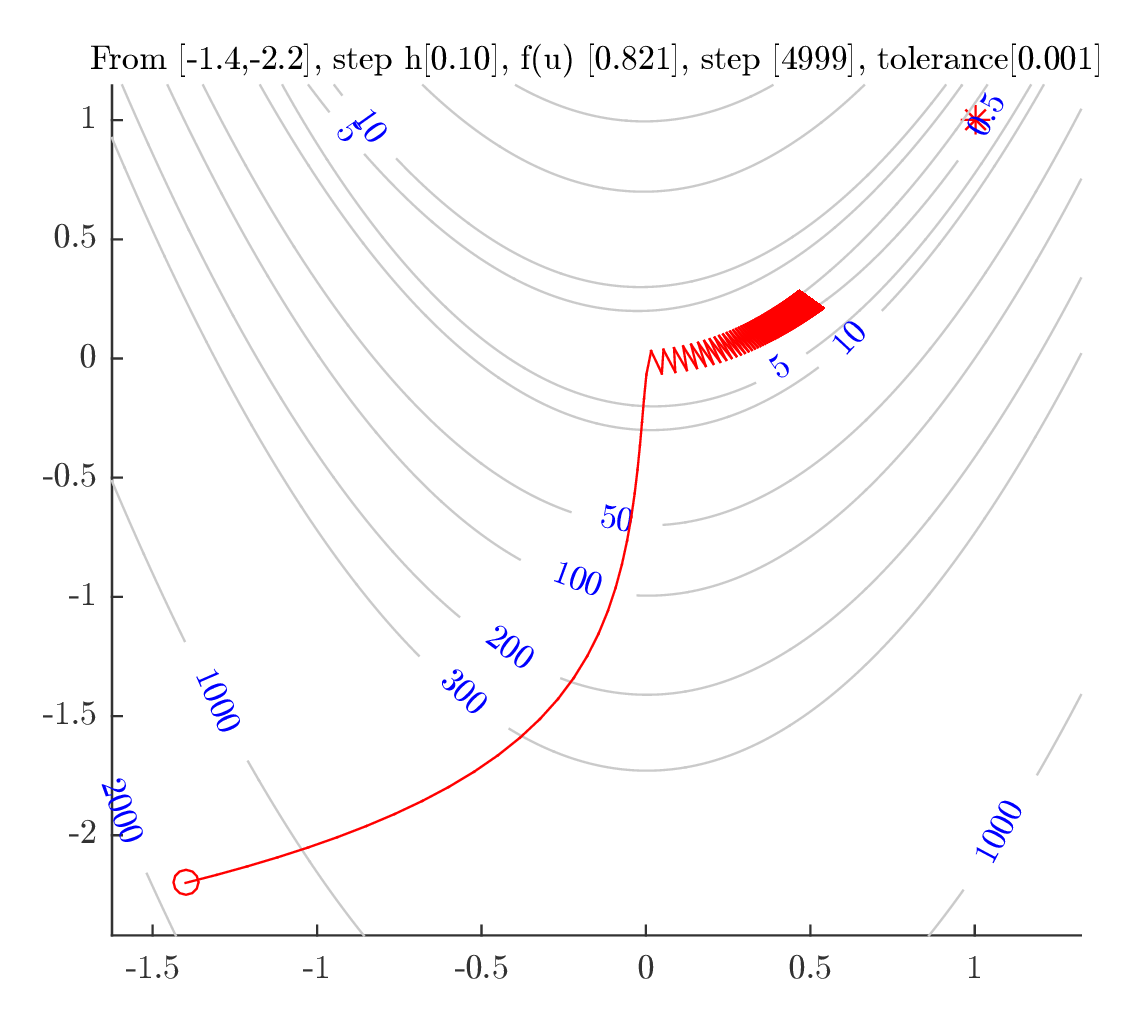
Starting from \((-1.4,-2.2)\)
| step size |
number of iterations to converge |
| optimal |
537 |
| \(0.1\) |
Did not converge within maximum iteration limit |
| \(0.05\) | Did not converge within maximum iteration limit, but stopped closer to \(u^{\ast }\) than the above case using \(h=0.1\) |
| \(0.01\) |
Did not converge within maximum iteration limit, but stopped closer to \(u^{\ast }\) than the above case using \(h=0.05\) |
The following plots show the path used in the above tests. Similar observation is seen as with the last starting point. In conclusion: One should use an optimal step size even though the optimal step requires more CPU time.


A program was written to automate the search for arbitrary \(n\). For example, for \(n=3\)\begin{align*} J\left ( u\right ) & =100\left ( u_{2}-u_{1}^{2}\right ) ^{2}+\left ( 1-u_{1}\right ) ^{2}+100\left ( u_{3}-u_{2}^{2}\right ) ^{2}+\left ( 1-u_{2}\right ) ^{2}\\ \nabla J\left ( u\right ) & =\begin{bmatrix} \frac{\partial J}{\partial u_{1}}\\ \frac{\partial J}{\partial u_{2}}\\ \frac{\partial J}{\partial u_{3}}\end{bmatrix} =\begin{bmatrix} -400\left ( u_{2}-u_{1}^{2}\right ) u_{1}-2\left ( 1-u_{1}\right ) \\ 200\left ( u_{2}-u_{1}^{2}\right ) -400\left ( u_{3}-u_{2}\right ) u_{2}-2\left ( 1-u_{2}\right ) \\ 200\left ( u_{3}-u_{2}^{2}\right ) \end{bmatrix} \end{align*}
And for \(n=4\)\begin{align*} J\left ( u\right ) & =100\left ( u_{2}-u_{1}^{2}\right ) ^{2}+\left ( 1-u_{1}\right ) ^{2}+100\left ( u_{3}-u_{2}^{2}\right ) ^{2}+\left ( 1-u_{2}\right ) ^{2}+100\left ( u_{4}-u_{3}^{2}\right ) ^{2}+\left ( 1-u_{3}\right ) ^{2}\\ \nabla J\left ( u\right ) & =\begin{bmatrix} \frac{\partial J}{\partial u_{1}}\\ \frac{\partial J}{\partial u_{2}}\\ \frac{\partial J}{\partial u_{3}}\\ \frac{\partial J}{\partial u_{4}}\end{bmatrix} =\begin{bmatrix} -400\left ( u_{2}-u_{1}^{2}\right ) u_{1}-2\left ( 1-u_{1}\right ) \\ 200\left ( u_{2}-u_{1}^{2}\right ) -400\left ( u_{3}-u_{2}^{2}\right ) u_{2}-2\left ( 1-u_{2}\right ) \\ 200\left ( u_{3}-u_{2}^{2}\right ) -400\left ( u_{4}-u_{3}^{2}\right ) u_{3}-2\left ( 1-u_{3}\right ) \\ 200\left ( u_{4}-u_{3}^{2}\right ) \end{bmatrix} \end{align*}
The pattern for \(\nabla J(u)\) is now clear. Let \(i\) be the row number of \(\nabla J\left (u\right ) \), where \(i=1\cdots N\), then the following will generate the gradient vector for any \(N\)\[ \nabla J\left ( u\right ) =\begin{bmatrix} \frac{\partial J}{\partial u_{i}}\\ \frac{\partial J}{\partial u_{i}}\\ \vdots \\ \frac{\partial J}{\partial u_{i}}\\ \frac{\partial J}{\partial u_{i}}\end{bmatrix} =\begin{bmatrix} -400\left ( u_{i+1}-u_{i}^{2}\right ) u_{i}-2\left ( 1-u_{i}\right ) \\ 200\left ( u_{i}-u_{i-1}^{2}\right ) -400\left ( u_{i+1}-u_{i}^{2}\right ) u_{i}-2\left ( 1-u_{i}\right ) \\ \vdots \\ 200\left ( u_{i}-u_{i-1}^{2}\right ) -400\left ( u_{i+1}-u_{i}^{2}\right ) u_{i}-2\left ( 1-u_{i}\right ) \\ 200\left ( u_{i}-u_{i-1}^{2}\right ) \end{bmatrix} \] The program implements the above to automatically generates \(\nabla J\left ( u\right ) \) and \(J\left ( u\right ) \) for any \(N\), then perform the search using steepest descent as before. The function that evaluates \(J(u)\) is the following
And the function that evaluates \(\nabla J(u)\) is the following
Two runs were made. One using fixed step size \(h=0.01\), and one using optimal step size. Both started from the same point \((-2,-2,\dots ,-2)\). Each time \(N\) was increased and the CPU time recorded. The same convergence criteria was used: \(| \nabla J(u)| \leq 0.0001\) and a maximum iteration limit of \(10^6\).
Only the CPU time used for the steepest descent call was recorder.
A typical run is given below. An example of the command used for \(N=8\) is
The program nma_HW4_problem_2_part_b_CPU was run in increments of \(20\) up to \(N=1000\). Here is the final result.

Discussion of result The fixed step size \(h=0.01\) was selected arbitrarily to compare against. Using fixed step size almost always produced oscillation when the search was near the optimal point and the search would stop.
Using an optimal step size, the search took longer time, as can be seen from the above plot, but it was reliable in that it converged, but at a very slow rate when it was close to the optimal point.
Almost all of the CPU time used was in the line search when using optimal search. This additional computation is the main difference between the fixed and optimal step size method.
In fixed step, \(|\nabla J(u)|\) was evaluated once at each step, while in optimal search, in addition to this computation, the function \(J(u)\) itself was also evaluated repeated times at each step inside the golden section line search. However, even though the optimal line search took much more CPU time, it converged much better than the fixed step size search did.
Using optimal line search produces much better convergence, at the cost of using much more CPU time.
The plot above shows that with fixed step size, CPU time grows linearly with the \(N\) while with optimal step size, the CPU time grew linearly but at a much larger slope, indicating it is more CPU expensive to use.


