
The following is diagram of the model of the problem to solve

The ANSYS APDL (input file) listing was provided to us to use and is given in the text file below for reference
The following 4 modal frequencies were generated by ANSYS after running the above APDL file.
| mode | Mode number | Frequency (Hz) |
| transverse | 1 | \(9.4438\) |
| torsional | 2 | \(34.272\) |
| transverse | 3 | \(111.41\) |
| longitudinal | 4 | \(420.31\) |
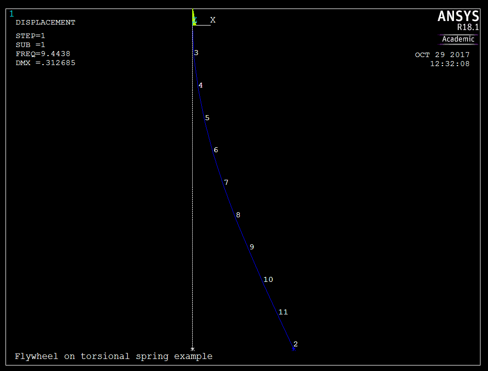
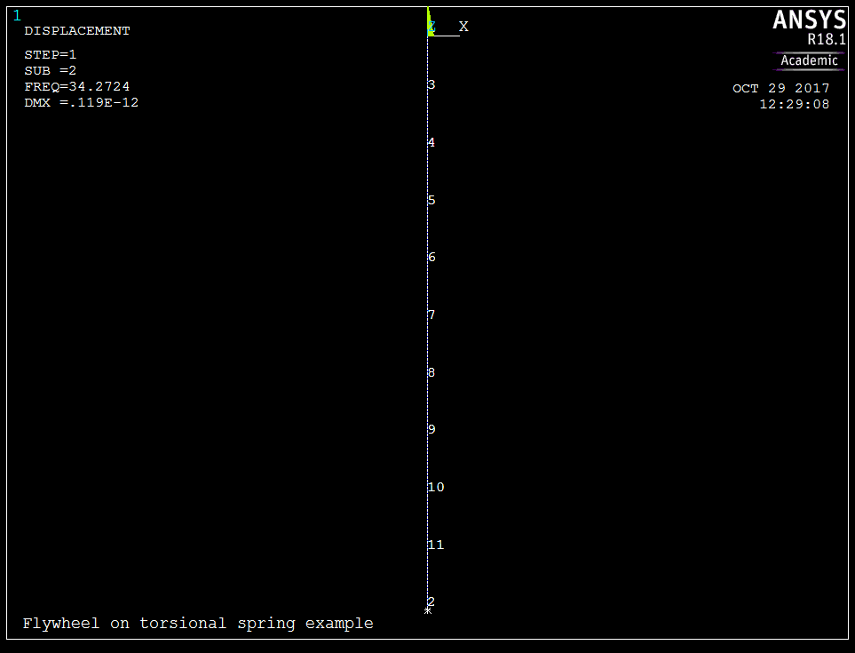
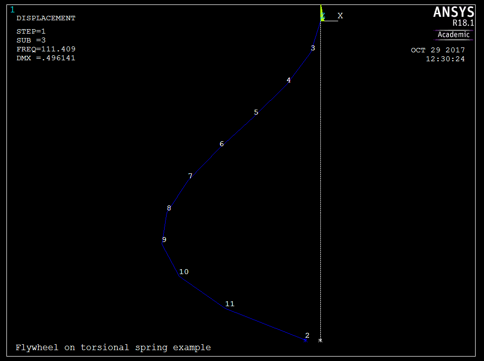
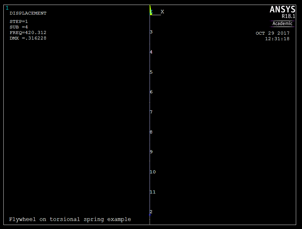
The modal shapes were then plotted using ANSYS. They are given below for each mode
The system parameters are
Total U displacement by ANSYS for mode 1 is
Total ROT displacement by ANSYS for mode 1 is
Total U displacement by ANSYS for mode 2 is
Total ROT displacement by ANSYS for mode 2 is
Total U displacement by ANSYS for mode 3 is
Total ROT displacement by ANSYS for mode 3 is
Total U displacement by ANSYS for mode 4 is
And total ROT displacement by ANSYS for mode 4 is
To verify ANSYS solution, this was solved in two ways. By taking into account the mass \(m\) of the pipe and then by ignoring the mass \(m\). Both hand solutions are given below. ANSYS do not take the mass of the pipe into account, since it was not told the density of the pipe material in the APDL input file. The first solution below is the recommend one to use to compare the ANSYS result against and it the method which gave more agreement with ANSYS result.
First solution. Not accounting for mass of pipe
Finding the longitudinal (axial) natural frequency.
Using \(k_{eq}=\frac{AE}{L}\) where \(A\) is the cross sectional area of the pipe and \(L\) is the pipe length and using \(m_{eq}=M\), then the longitudinal natural frequency is \begin{equation} \omega _{n}=\sqrt{\frac{k_{eq}}{m_{eq}}}=\sqrt{\frac{AE}{LM}}\tag{1} \end{equation} The cross sectional area of the pipe is\begin{align*} A & =\frac{\pi }{4}\left ( D_{o}^{2}-D_{i}^{2}\right ) \\ & =\frac{\pi }{4}\left ( \left ( 0.04\right ) ^{2}-\left ( 0.034\right ) ^{2}\right ) \\ & =3.487\,2\times 10^{-4}\text{ m}^{2} \end{align*}
The length of pipe is \(1~\)meter and \(M=10\) kg. Equation (1) becomes\begin{align*} \omega _{n} & =\sqrt{\frac{\left ( 3.487\,2\times 10^{-4}\right ) \left ( 200\times 10^{9}\right ) }{\left ( 1\right ) \left ( 10\right ) }}\\ & =2640.9\text{ rad/sec} \end{align*}
The cycle frequency is\begin{align*} f_{n} & =\frac{\omega _{n}}{2\pi }\\ & =\frac{2640.9}{2\pi }\\ & =420.31\text{ Hz} \end{align*}
ANSYS gives \(420.31\) Hz. So the error is \(0\)\(.\)
Finding the torsional natural frequency.
Torsional stiffness \(k_{t}\) is\[ k_{t}=\frac{GJ}{L}\] Where \(G\) is the shear modulus (given in handout), and \(J\) is the polar area moment of inertia of the cross section given by\begin{align*} J & =\frac{\pi }{32}\left ( D_{o}^{4}-D_{i}^{4}\right ) \\ & =\frac{\pi }{32}\left ( 0.04^{4}-0.034^{4}\right ) \\ & =1.201\,3\times 10^{-7}\ \text{m}^{4} \end{align*}
Therefore\[ k_{t}=\frac{\left ( 77.2\times 10^{9}\right ) \left ( 1.201\,3\times 10^{-7}\right ) }{1}=9274\text{ N-m per radian}\] The equivalent mass is just the mass moment of inertia of the flywheel \(\frac{1}{2}Mr_{f}^{2}\) (since the pipe assumed to have no mass). Hence the torsional frequency is\begin{align*} \omega & =\sqrt{\frac{k_{t}}{\frac{1}{2}Mr_{f}^{2}}}\\ & =\sqrt{\frac{9274}{\frac{1}{2}\left ( 10\right ) \left ( 0.2\right ) ^{2}}}\\ & =215.34\text{ rad/sec} \end{align*}
Therefore the torsional frequency in Hz is\begin{align*} f & =\frac{215.34}{2\pi }\\ & =34.272\text{ hz} \end{align*}
ANSYS gives this as \(34.272\) Hz. The the error is \(0\)\(.\)
Finding the transverse natural frequency:
Using \(k=\frac{3EI}{L^{3}}\) and \(M=10\). Where \(I\) is the area moment of inertia given by\begin{align*} I & =\frac{\pi }{64}\left ( D_{o}^{4}-D_{i}^{4}\right ) \\ & =\frac{\pi }{64}\left ( 0.04^{4}-0.034^{4}\right ) \\ & =6.0066\times 10^{-8}\ \text{m}^{4} \end{align*}
The transverse natural frequency is therefore\begin{align*} \omega & =\sqrt{\frac{3EI}{ML^{3}}}\\ & =\sqrt{\frac{3\left ( 200\times 10^{9}\right ) \left ( 6.0066\times 10^{-8}\right ) }{\left ( 10\right ) \left ( 1\right ) ^{3}}}\\ & =60.033\text{ rad/sec} \end{align*}
Hence\[ f_{n}=\frac{60.033}{2\pi }=9.5545\text{ Hz}\] ANSYS gives \(9.4438\) for the first transverse natural frequency. Hence error is \(\left ( \frac{\allowbreak \left \vert 9.4438-9.5545\right \vert }{9.4438}\right ) 100=1.1722\,\%\)
Summary of results
| mode | ANSYS result | Hand calculation | %error |
| First transverse | \(9.4438\) | \(9.554\,5\) | \(1.1722\,\%\) |
| First torsional | \(34.272\) | \(34.272\) | \(0\%\) |
| First longitudinal (axial) | \(420.31\) | \(420.31\) | \(0\%\) |
All the analytical solutions gave exact agreement with ANSYS except for the transverse case. The transverse case uses stiffness \(\frac{3EI}{L^{3}}\) due to load at end of fixed-free beam. This does not account for bending rotation in the beam. That is why ANSYS result is more accurate, as its finite elements account for the small bending associated with the transverse vibration. In the other two cases (Torsional and axial), there is no associated bending, hence the solutions agree.
Second solution. Accounting for mass of pipe
Finding the longitudinal natural frequency.
Following the example given in the textbook, at page 715, the (first) longitudinal natural frequency is found to be\begin{equation} \omega _{1}=\frac{\alpha _{1}\sqrt{\frac{E}{\rho }}}{L} \tag{E.4} \end{equation} Where \(\alpha _{1}\) is the (first) root of \[ \alpha \tan \alpha =\beta \] Where \(\beta \) is the mass ratio \(\beta =\frac{m}{M}\) where \(m\) is mass of pipe and \(M\) is end mass (flywheel). To find mass of pipe \(m\), using steel density \(\rho =7800\) kg/m\(^{3}\), we first find the volume of the pipe.
Let \(D_{i}\) be the inner diameter and \(D_{o}\) the outer diameter. \(D_{o}=0.04\) meter and \(D_{i}=0.04-2\left ( 0.003\right ) =\allowbreak 0.034\) meter\(\,\,\), therefore the cross sectional area of the pipe is\begin{align*} A & =\frac{\pi }{4}\left ( D_{o}^{2}-D_{i}^{2}\right ) \\ & =\frac{\pi }{4}\left ( \left ( 0.04\right ) ^{2}-\left ( 0.034\right ) ^{2}\right ) \\ & =3.487\,2\times 10^{-4}\text{ m}^{2} \end{align*}
And since length of pipe is \(1~\)meter, the mass of pipe is \begin{align*} m & =\rho AL\\ & =\left ( 7800\right ) \left ( 3.487\,2\times 10^{-4}\right ) \left ( 1\right ) \\ & =2.72\text{ kg.} \end{align*}
The mass at the end is given as \(M=10\) kg. Therefore the mass ratio \[ \beta =\frac{m}{M}=\frac{2.72}{10}=0.272\, \] To find \(\alpha _{1}\) we now need to solve \(\alpha _{1}\tan \alpha _{1}=0.272\). This was solved numerical using root finder. The first root was found to be\[ \alpha _{1}=0.499 \] Therefore from equation E.4 in textbook (page 715) \begin{align*} \omega _{1} & =\frac{\alpha _{1}c}{L}\\ & =\frac{\alpha _{1}\sqrt{\frac{E}{\rho }}}{L}\\ & =\frac{\left ( 0.499\right ) \sqrt{\frac{200\times 10^{9}}{7800}}}{1}\\ & =2526.8\text{ rad/sec} \end{align*}
Therefore\begin{align*} f_{1} & =\frac{\omega _{1}}{2\pi }\\ & =\frac{2526.8}{2\pi }\\ & =402.15\text{ Hz} \end{align*}
ANSYS gives \(420.31\) Hz. So the error is \(\left ( \frac{420.31-402.\,\allowbreak 15}{420.31}\right ) 100=4.321\%\)
Finding the torsional natural frequency.
\(k_{t}\) is\[ k_{t}=\frac{GJ}{L}\] Where \(G\) is the shear modulus (given in handout), and \(J\) is the polar area moment of inertia of the cross section given by\begin{align*} J & =\frac{\pi }{32}\left ( D_{o}^{4}-D_{i}^{4}\right ) \\ & =\frac{\pi }{32}\left ( 0.04^{4}-0.034^{4}\right ) \\ & =1.201\,3\times 10^{-7}\ \text{m}^{4} \end{align*}
Hence\[ k_{t}=\frac{\left ( 77.2\times 10^{9}\right ) \left ( 1.201\,3\times 10^{-7}\right ) }{1}=9274 \] To find equivalent mass, using kinetic energy method\begin{equation} \frac{1}{2}I_{flywheel}\dot{\theta }^{2}+\frac{1}{2}I_{pipe}\dot{\theta }^{2}=\frac{1}{2}I_{eq}\dot{\theta }^{2} \tag{1} \end{equation} For a hollow pipe, where now \(m\) is replaced by \(\frac{1}{3}m\) from continuous system derivation. \begin{align*} I_{pipe} & =\frac{1}{2}\left ( \frac{1}{3}m\right ) \left ( \left ( \frac{D_{o}}{2}\right ) ^{2}+\left ( \frac{D_{i}}{2}\right ) ^{2}\right ) \\ & =\frac{1}{24}m\left ( D_{o}^{2}+D_{i}^{2}\right ) \end{align*}
And for the flywheel, \(I_{fly}=\frac{1}{2}Mr_{f}^{2}\) where \(r_{f}=0.2\) meter. Hence from (1) \begin{align*} I_{eq} & =\frac{1}{2}Mr_{f}^{2}+\frac{1}{24}m\left ( D_{o}^{2}+D_{i}^{2}\right ) \\ & =\frac{1}{2}\left ( 10\right ) \left ( 0.2\right ) ^{2}+\frac{1}{24}\left ( 2.72\right ) \left ( 0.04^{2}+0.034^{2}\right ) \\ & =0.20031\text{ kg-m}^{2} \end{align*}
Hence the torsional frequency is\begin{align*} \omega & =\sqrt{\frac{k_{t}}{I_{eff}}}\\ & =\sqrt{\frac{9274}{0.20031}}\\ & =215.17\text{ rad/sec} \end{align*}
Therefore the torsional frequency in Hz is\begin{align*} f & =\frac{215.17}{2\pi }\\ & =34.245\text{ hz} \end{align*}
ANSYS gives this as \(34.272\) Hz. The the error is \(\left ( \frac{34.272-34.\,245}{34.272}\right ) 100=0.079\%\)
Finding the transverse natural frequency:
From textbook, table 8.15 page 726, it gives for fixed-end beam the value \(\beta _{1}L=1.875104\). But since there is a mass attach to the end in our problem, I did not know how to add this using the table.
So I used the other method we used before, which is the Rayleigh energy method, where we assume motion is simple harmonic motion. Taking the displacement as the transverse motion of the free end of the pipe (where the large mass is attached), measured from equilibrium then the kinetic energy is\[ T=\frac{1}{2}\overset{m_{eq}}{\overbrace{\left ( M+0.23m\right ) }}\dot{x}^{2}\] Where we added \(0.23m\), where \(m\) is the mass of the pipe, since this is continuous mass. For the potential energy, we use the stiffness formula for the fixed-free beam which is \(k=\frac{3EI}{L^{3}}\), hence\[ U=\frac{1}{2}kx^{2}\] Now, assuming \(x=X\sin \omega _{n}t\), then \(\dot{x}=X\omega _{n}\cos \omega _{n}t\). Therefore when\[ U_{\max }=T_{\max }\] We obtain \begin{align} \frac{1}{2}\frac{3EI}{L^{3}}X^{2} & =\frac{1}{2}\left ( M+0.23m\right ) \left ( X\omega _{n}\right ) ^{2}\nonumber \\ \frac{3EI}{L^{3}} & =\left ( M+0.23m\right ) \omega _{n}^{2}\nonumber \\ \omega _{n}^{2} & =\frac{3EI}{L^{3}\left ( M+0.23m\right ) }\nonumber \\ \omega _{n} & =\sqrt{\frac{3EI}{L^{3}\left ( M+0.23m\right ) }} \tag{1} \end{align}
Where \(I\) now is the area moment of inertia2 is given by\begin{align*} I & =\frac{\pi }{64}\left ( D_{o}^{4}-D_{i}^{4}\right ) \\ & =\frac{\pi }{64}\left ( 0.04^{4}-0.034^{4}\right ) \\ & =6.006\,6\times 10^{-8}\ \text{m}^{4} \end{align*}
And\begin{align*} M+0.23m & =10+0.23\left ( 2.72\right ) \\ & =10.626\text{ kg} \end{align*}
Substituting the numerical values in (1) gives\begin{align*} \omega _{n} & =\sqrt{\frac{3\left ( 200\times 10^{9}\right ) \left ( 6.006\,6\times 10^{-8}\right ) }{10.626}}\\ & =58.239\text{ rad/sec} \end{align*}
Hence\[ f_{n}=\frac{58.239}{2\pi }=9.269\text{ Hz}\] ANSYS gives \(9.4438\) for the first transverse natural frequency. Hence error is \(\left ( \frac{\allowbreak 9.4438-9.269}{9.4438}\right ) 100=1.851\,\%\)
Summary of results
| mode | ANSYS result | Hand calculation | %error |
| First transverse | \(9.4438\) | \(9.269\) | \(1.851\,\%\) |
| First torsional | \(34.272\) | \(34.245\) | \(0.079\%\) |
| First longitudinal | \(420.31\) | \(402.15\) | \(4.321\%\) |
Comparing the above table to the first solution, it shows that ignoring the mass of the pipe gave result which agree with ANSYS result much better. This is because ANSYS did not take into the account the mass of the pipe. It will be interesting exercise to find how to change the APDL input file to make ANSYS account for the mass of the pipe and then compare the above results with ANSYS.

The first step is to determine the natural frequency \(\omega _{n}\) for the transverse vibration. Rayleigh energy method was used to find the transverse frequency. Taking the displacement as the transverse motion of the free end of the sigpost (where the large mass \(M\) is attached), measured from equilibrium, then the kinetic energy is\[ T=\frac{1}{2}\overset{m_{eq}}{\overbrace{\left ( M+0.23m\right ) }}\dot{x}^{2}\] \(m\) is the mass of the sigpost. For the potential energy, the bending stiffness formula for the fixed-free beam with load at the end was used, which is\[ k=\frac{3EI}{L^{3}}\] The potential energy is therefore\[ U=\frac{1}{2}kx^{2}\] Assuming \(x=X\sin \omega _{n}t\), then \(\dot{x}=X\omega _{n}\cos \omega _{n}t\). Using\[ U_{\max }=T_{\max }\] Then the above reduces to\begin{align} \frac{1}{2}\left ( \frac{3EI}{L^{3}}\right ) X^{2} & =\frac{1}{2}\left ( M+0.23m\right ) \left ( X\omega _{n}\right ) ^{2}\nonumber \\ \frac{3EI}{L^{3}} & =\left ( M+0.23m\right ) \omega _{n}^{2}\nonumber \\ \omega _{n}^{2} & =\frac{3EI}{L^{3}\left ( M+0.23m\right ) }\nonumber \\ \omega _{n} & =\sqrt{\frac{3EI}{L^{3}\left ( M+0.23m\right ) }}\tag{1} \end{align}
\(I\) is the area moment of inertia of the pipe cross section. Since \(D_{o}=0.25\) m and \(D_{i}=0.2\) m, then\begin{align*} I & =\frac{\pi }{64}\left ( D_{o}^{4}-D_{i}^{4}\right ) \\ & =\frac{\pi }{64}\left ( 0.25^{4}-0.2^{4}\right ) \\ & =1.132\,1\times 10^{-4}\ \text{m}^{4} \end{align*}
\(M=200\) kg, and \(L=10\) meter. Using \(\rho _{steel}g=76500\) N/m\(^{3}\) and \(E=207\times 10^{9}\) Pa. To find the mass \(m\) of the post, the cross sectional area is first found\begin{align*} A & =\frac{\pi }{4}\left ( D_{o}^{2}-D_{i}^{2}\right ) \\ & =\frac{\pi }{4}\left ( 0.25^{2}-0.2^{2}\right ) \\ & =0.017671\text{ m}^{2} \end{align*}
Hence the mass \(m\) is\begin{align*} m & =\frac{\left ( \rho _{steel}g\right ) }{g}AL\\ & =\frac{76500}{9.81}\left ( 0.017671\right ) \left ( 10\right ) \\ & =1378\text{ kg} \end{align*}
Substituting the numerical values in (1) gives\begin{align*} \omega _{n} & =\sqrt{\frac{3EI}{L^{3}\left ( M+0.23m\right ) }}\\ & =\sqrt{\frac{3\left ( 207\times 10^{9}\right ) \left ( 1.132\,1\times 10^{-4}\right ) }{\left ( 10\right ) ^{3}\left ( 200+0.23\left ( 1378\right ) \right ) }}\\ & =11.662\text{ rad/sec} \end{align*}
Or \[ f_{n}=\frac{11.662\,}{2\pi }\] Therefore\[ \fbox{$f_n=1.856\,1$ Hz}\]
Maximum steady state displacement occurs at resonance. This is when the frequency of vortex shedding is the same as the natural frequency \(f_{n}\) of the post found above. Using Strouhal formula\[ v=\frac{f_{n}D_{o}}{S}\] Where in the above \(v\) is the wind velocity and the vortex shedding frequency is set to be the natural frequency in order to obtain the maximum displacement. Assume \(S=0.21\) gives\[ v=\frac{\left ( 1.856\,1\right ) \left ( 0.25\right ) }{0.21}\] Hence\[ \fbox{$v=2.2096$ m/s}\] Checking Reynold number\[ \operatorname{Re}=\frac{vD_{o}\rho _{air}}{\mu }\] \(\rho _{air}\) is density of air and \(\mu \) is viscosity of air. Using the numerical values given the above becomes\begin{align*} \operatorname{Re} & =\frac{\left ( 2.209\,6\right ) \left ( 0.25\right ) \left ( 1.2\right ) }{\left ( 1.8\times 10^{-5}\right ) }\\ & =36827 \end{align*}
Since \(400\leq \operatorname{Re}\leq 300000\) then the assumption of Strouhal \(S=0.21\) was valid.
The lateral force exerted by the wind on the sigpost is given by\begin{align*} F\left ( t\right ) & =\frac{1}{2}c\rho _{air}v^{2}A\sin \omega t\\ & =F_{0}\sin \omega t \end{align*}
Where \(c\approx 1\) for cylinder and \(v\) is the wind speed found in last part and \(A\) is the projected area \(A=D_{o}L\). Hence\begin{align*} F_{0} & =\frac{1}{2}c\rho _{air}v^{2}A\\ & =\frac{1}{2}\left ( 1.2\right ) \left ( 2.2096\right ) ^{2}\left ( 0.25\right ) \left ( 10\right ) \\ & =7.3235\text{ N} \end{align*}
Using the steady state displacement formula for damped single degree of freedom system, which is\[ y_{ss}=\frac{F_{0}}{k}\frac{1}{\sqrt{\left ( 1-r^{2}\right ) ^{2}+\left ( 2\xi r\right ) ^{2}}}\] Where \(F_{0}\) is total force from the wind over the whole span. Assuming this force acts at the end of a fixed-free beam (This is an over estimation. The wind force actually acts over the whole length of the sigpost, but it is now taken as acting on the end). Therefore \(k=\frac{3EI}{L^{3}}\) can be used based on this. Since \(r=1\) (resonance) and \(\xi =0.1\), then \(y_{ss}\) is now evaluated\begin{align*} y_{ss} & =\frac{F_{0}}{k}\frac{1}{\sqrt{4\xi ^{2}}}\\ & =\frac{F_{0}L^{3}}{3EI}\frac{1}{2\xi }\\ & =\frac{\left ( 7.3235\right ) \left ( 10\right ) ^{3}}{3\left ( 207\times 10^{9}\right ) \left ( 1.132\,1\times 10^{-4}\right ) }\frac{1}{2\left ( 0.1\right ) }\\ & =5.208\,5\times 10^{-4}\text{ meter} \end{align*}
Or\[ y_{ss}\approx 0.5\text{ mm}\]