;
;
;
 ;
;
 ;
;
 ;
;
 ;
;
 ;
;
A Matrix \(\mathbb{C} \) is rank deficient if there exist a non-zero vector \(\mathbf{\alpha }\) such that \(\mathbb{C} \mathbf{\alpha }=\mathbf{0}\). This means that the Null space of \(\mathbb{C} \) is not empty. The idea of the proof is to apply this to the controllability matrix itself to check if \(\mathbb{C} \) is full rank or not. The left null space is used instead. If the left null space of \(\mathbb{C} \) is not empty, this implies Null space of \(\mathbb{C} \) is also not empty, hence \(\mathbb{C} \) is rank deficient, which gives the proof.
The first step is to find \(\mathbb{C} \)\[\mathbb{C} =\begin{bmatrix} B & AB & A^{2}B & \cdots & A^{n-1}B \end{bmatrix} \] \(\mathbf{\alpha }^{T}\mathbb{C} \) is now found to see if it produces zero row vector. If it does, then the left null space of \(\mathbb{C} \) is not empty.\[ \mathbf{\alpha }^{T}\mathbb{C} =\mathbf{\alpha }^{T}\begin{bmatrix} B & AB & A^{2}B & \cdots & A^{n-1}B \end{bmatrix} \] But \(\mathbf{\alpha }^{T}\) pre-multiplied by a matrix is \(\mathbf{\alpha }^{T}\) pre-multiplied by each one of the columns of the matrix. The above becomes \begin{align*} \mathbf{\alpha }^{T}\mathbb{C} & =\begin{bmatrix} \mathbf{\alpha }^{T}B & \mathbf{\alpha }^{T}AB & \mathbf{\alpha }^{T}A^{2}B & \cdots & \mathbf{\alpha }^{T}A^{n-1}B \end{bmatrix} \\ & =\begin{bmatrix} \mathbf{\alpha }^{T}B & \left ( \mathbf{\alpha }^{T}A\right ) B & \left ( \mathbf{\alpha }^{T}A\right ) AB & \cdots & \left ( \mathbf{\alpha }^{T}A\right ) A^{n-2}B \end{bmatrix} \end{align*}
\(\mathbf{\alpha }^{T}A\) is replaced by \(\lambda \mathbf{\alpha }^{T}\) in the above giving\begin{align*} \mathbf{\alpha }^{T}\mathbb{C} & =\begin{bmatrix} \mathbf{\alpha }^{T}B & \left ( \lambda \mathbf{\alpha }^{T}\right ) B & \left ( \lambda \mathbf{\alpha }^{T}\right ) AB & \cdots & \left ( \lambda \mathbf{\alpha }^{T}\right ) A^{n-2}B \end{bmatrix} \\ & =\begin{bmatrix} \mathbf{\alpha }^{T}B & \lambda \left ( \mathbf{\alpha }^{T}B\right ) & \lambda \left ( \mathbf{\alpha }^{T}A\right ) B & \cdots & \left ( \lambda \mathbf{\alpha }^{T}A\right ) A^{n-3}B \end{bmatrix} \end{align*}
Applying \(\mathbf{\alpha }^{T}A=\lambda \mathbf{\alpha }^{T}\) again on the above\[ \mathbf{\alpha }^{T}\mathbb{C} =\begin{bmatrix} \mathbf{\alpha }^{T}B & \lambda \left ( \mathbf{\alpha }^{T}B\right ) & \lambda \lambda \mathbf{\alpha }^{T}B & \cdots & \left ( \lambda \lambda \mathbf{\alpha }^{T}A\right ) A^{n-4}B \end{bmatrix} \] This process is continued until the final result is\[ \mathbf{\alpha }^{T}\mathbb{C} =\begin{bmatrix} \left ( \mathbf{\alpha }^{T}B\right ) & \lambda \left ( \mathbf{\alpha }^{T}B\right ) & \lambda ^{2}\left ( \mathbf{\alpha }^{T}B\right ) & \cdots & \lambda ^{n-1}\left ( \mathbf{\alpha }^{T}B\right ) \end{bmatrix} \] Letting \(\mathbf{\alpha }^{T}B=0\) in the above results in\[ \mathbf{\alpha }^{T}\mathbb{C} =\begin{bmatrix} 0 & 0 & 0 & \cdots & 0 \end{bmatrix} \] Hence\[ \mathbf{\alpha }^{T}\mathbb{C} =\mathbf{0}^{T}\] Since \(\mathbf{\alpha }\) is not zero then the above implies the left null space of \(\mathbb{C} \) is not empty. Taking the transpose of both sides gives\begin{align*} \left ( \mathbf{\alpha }^{T}\mathbb{C} \right ) ^{T} & =\mathbf{0}\\\mathbb{C} ^{T}\mathbf{\alpha } & =\mathbf{0} \end{align*}
The null space of the transpose of \(\mathbb{C} \) is not empty. Hence \(\mathbb{C} ^{T}\) is not full rank which means \(\mathbb{C} \) is is not full rank (Transposing a matrix does not change its rank). This implies \(\left ( A,B\right ) \) is not controllable by definition.
A function sequence \(f_{n}\) on \(D\) is said to converge pointwise to \(f\) if \(\lim _{n\rightarrow \infty }f_{n}\left ( t\right ) \) exist for each \(t\) in \(D\). This means, not only the limit needs to be found, if it exist, but there should be a limit for each \(t\) in the interval the function is defined over. If for even a single \(t_{0}\) there is no limit, then the function does not converge pointwise. \[ \lim _{n\rightarrow \infty }\frac{t^{2}}{1+nt}=t^{2}\lim _{n\rightarrow \infty }\frac{1}{1+nt}\] When \(t=0\) the limit is zero. For all other values, \(0<t<\infty \) the limit is \(t^{2}\frac{1}{\infty }=0\). So the limit exists for each \(t\). The pointwise limit is the function \(f^{\ast }\left ( t\right ) =0\).
Now to find if the sequence converges uniformly. A function sequence \(f_{n}\left ( t\right ) \) is uniformly convergent on \(D\) if for each \(\epsilon >0\) one can find an integer \(N\) such that \(\left \Vert f_{n}-f\right \Vert <\epsilon \) and all \(n\geq N\) and each \(t\) in \(D.\)The integer \(N\) here depends only on \(\epsilon \) and does not depend on \(t\). For pointwise convergence, \(N\) depends on both \(t\) and \(\epsilon .\)
Since the sequence convergence pointwise to \(f^{\ast }\left ( t\right ) =0\) then one needs to show that\[ \left \Vert f_{n}-f\right \Vert _{I}=\sup _{0\leq t<\infty }\left \vert f_{n}\left ( t\right ) -f^{\ast }\left ( t\right ) \right \vert \]
goes to zero as \(n\rightarrow \infty \). But \(f^{\ast }\left ( t\right ) =0\) from above, hence\begin{align*} \left \Vert f_{n}-f\right \Vert _{I} & =\sup _{0\leq t<\infty }\left \vert f_{n}\left ( t\right ) \right \vert \\ & =\sup _{0\leq t<\infty }\left \vert \frac{t^{2}}{1+nt}\right \vert \end{align*}
To find the maximum of \(f_{n}\left ( t\right ) =\frac{t^{2}}{1+nt}\), the equation \(f_{n}^{\prime }\left ( t\right ) =0\) is first solved for \(t\) \begin{align*} \frac{d}{dt}\left ( \frac{t^{2}}{1+nt}\right ) & =0\\ \frac{t\left ( 2+nt\right ) }{(1+nt)^2} & =0 \end{align*}
Hence \(t(2+nt)=0\) gives the solutions \(t=0\) and \(t=-\frac{2}{n}\). When \(t=0\) then \(f_{n}\left ( 0\right ) =0\) and when \(t=-\frac{2}{n}\) then \(f_{n}\left ( -\frac{2}{n}\right ) =\frac{\left ( -\frac{2}{n}\right ) ^{2}}{1+n\left ( -\frac{2}{n}\right ) }=-\frac{4}{n^{2}}\)
The maximum of these is \(\frac{4}{n^{2}}\) in absolute terms. Hence \[ \sup _{0\leq t<\infty }\left \vert \frac{t^{2}}{1+nt}\right \vert =\frac{4}{n^{2}}\]
Therefore \[ \left \Vert f_{n}-f\right \Vert _{I}=\frac{4}{n^{2}}\]
Taking the limit \(n\rightarrow \infty \) gives\[ \lim _{n\rightarrow \infty }\left \Vert f_{n}-f\right \Vert _{I}=0 \] Since the limit is zero, then the sequence does convergences uniformly.
\(I={\displaystyle \int \limits _{0}^{1}} t\left ( 1-t^{2}\right ) ^{k}dt\) is first evaluated. This is done using substitution Let \(u=1-t^{2}\), hence \(du=-2tdt\). When \(t=0,u=1\) and when \(t=1,u=0\). Therefore the integral becomes\begin{align*} I & ={\displaystyle \int \limits _{1}^{0}} tu^{k}\frac{du}{-2t}\\ & =\frac{-1}{2}{\displaystyle \int \limits _{1}^{0}} u^{k}du\\ & =\frac{-1}{2}\left [ \frac{u^{k+1}}{k+1}\right ] _{1}^{0}\\ & =\frac{-1}{2\left ( k+1\right ) }\left [ 0-1\right ] \\ & =\frac{1}{2\left ( k+1\right ) } \end{align*}
Hence\begin{align*} \lim _{k\rightarrow \infty }{\displaystyle \int \limits _{0}^{1}} f_{k}\left ( t\right ) dt & =\lim _{k\rightarrow \infty }{\displaystyle \int \limits _{0}^{1}} k^{2}t\left ( 1-t^{2}\right ) ^{k}dt=\lim _{k\rightarrow \infty }k^{2}\frac{1}{2\left ( k+1\right ) }\\ & =\frac{1}{2}\left ( \lim _{k\rightarrow \infty }k+\lim _{k\rightarrow \infty }k^{2}\right ) \\ & =\infty \end{align*}
Let \(f^{\ast }\left ( t\right ) \) be the pointwise limit of \(f_{k}\left ( t\right ) \). At \(t=0\), \(\lim _{k\rightarrow \infty }f_{k}\left ( 0\right ) =0\) and at \(t=1\), \(\lim _{k\rightarrow \infty }f_{k}\left ( 1\right ) =0.\) For \(0<t<1\) \begin{align*} \lim _{k\rightarrow \infty }f_{k}\left ( t\right ) & =\lim _{k\rightarrow \infty }k^{2}t\left ( 1-t^{2}\right ) ^{k}\\ & =\lim _{k\rightarrow \infty }k^{2}te^{k\ln \left ( 1-t^{2}\right ) } \end{align*}
Since \(\,0<1-t^{2}<1\) for \(0<t<1\) then \(\ln \left ( 1-t^{2}\right ) \) is negative, hence \(e^{k\ln \left ( 1-t^{2}\right ) }\) will go to zero in the limit much faster than \(k^{2}\) going towards infinity. Hence\[ \lim _{k\rightarrow \infty }f_{k}\left ( t\right ) =0 \] This shows that the pointwise convergence is \(f^{\ast }\left ( t\right ) =0\)\(.\)Therefore \({\displaystyle \int \limits _{0}^{1}} f^{\ast }\left ( t\right ) dt=0\)
From the first part it was found that \(\lim _{k\rightarrow \infty }{\displaystyle \int \limits _{0}^{1}} f_{k}\left ( t\right ) dt=\infty \) and from the second part \({\displaystyle \int \limits _{0}^{1}} \lim _{k\rightarrow \infty }f_{k}\left ( t\right ) =0\)\(.\)It is clear the quantities are the not the same. To be able to move the limit inside the integral, the sequence must be uniformly convergent.
The above indirectly indicates that \(f_{k}\left ( t\right ) \) is not uniform convergent. This can be confirmed by trying to find the uniform convergence limit to show that it does not exist:\[ \left \Vert f_{k}-f\right \Vert _{I}=\max _{0\leq t\leq 1}\left \vert f_{k}\left ( t\right ) -f^{\ast }\left ( t\right ) \right \vert =\max _{0\leq t\leq 1}\left \vert f_{k}\left ( t\right ) \right \vert \]
Since \(f^{\ast }\left ( t\right ) =0\) identically. Hence
\[ \left \Vert f_{k}-f\right \Vert _{I}=\max _{0\leq t\leq 1}\left \vert k^{2}t\left ( 1-t^{2}\right ) ^{k}\right \vert \]
At \(t=0,\) \(f_{k}=0\) and at \(t=1,f_{k}\left ( 0\right ) =0\). The maximum value between zero and one is found from calculus:\begin{align*} f_{k}^{\prime }\left ( t\right ) & =0\\ k^{2}\left ( 1-t^{2}\right ) ^{k}-2k^{3}t^{2}\left ( 1-t^{2}\right ) ^{k-1} & =0\\ k\left ( 1-t^{2}\right ) ^{k-1}\left ( \left ( 1+2k\right ) t^{2}-1\right ) & =0 \end{align*}
The solution is \(t=\pm \frac{1}{\sqrt{1+2k}}\). Substituting this back into \(f_{k}\left ( t\right ) \) gives the value (using the positive root) \begin{align*} f_{_{k}\max } & =k^{2}t\left ( 1-t^{2}\right ) ^{k}\\ & =k^{2}\frac{1}{\sqrt{1+2k}}\left ( 1-\frac{1}{1+2k}\right ) ^{k} \end{align*}
Therefore
\[ \left \Vert f_{n}-f\right \Vert _{I}=\left \vert k^{2}\frac{1}{\sqrt{1+2k}}\left ( 1-\frac{1}{1+2k}\right ) ^{k}\right \vert \]
Taking the limit of the above as \(k\rightarrow \infty \) gives\begin{align*} \left \Vert f_{k}-f\right \Vert _{I} & =\lim _{k\rightarrow \infty }k^{2}\frac{1}{\sqrt{1+2k}}\left ( 1-\frac{1}{1+2k}\right ) ^{k}\\ & =\left ( \lim _{k\rightarrow \infty }k^{2}\frac{1}{\sqrt{1+2k}}\right ) \lim _{k\rightarrow \infty }\left ( 1-\frac{1}{1+2k}\right ) ^{k}\\ & =\left ( \lim _{k\rightarrow \infty }k^{2}\frac{1}{\sqrt{1+2k}}\right ) \lim _{k\rightarrow \infty }\left ( 1-\frac{\frac{1}{k}}{\frac{1}{k}+2}\right ) ^{k}\\ & =\left ( \lim _{k\rightarrow \infty }k^{2}\frac{1}{\sqrt{1+2k}}\right ) \frac{1}{\sqrt{e}}\\ & =\left ( \lim _{k\rightarrow \infty }\frac{1}{\sqrt{\frac{1}{k^{4}}+\frac{2}{k^{3}}}}\right ) \frac{1}{\sqrt{e}}\\ & =\left ( \frac{1}{0}\right ) \frac{1}{\sqrt{e}}\\ & =\infty \frac{1}{\sqrt{e}}\\ & =\infty \end{align*}
Therefore since the limit does not go to zero, then \(f_{k}\left ( t\right ) \) does not converge uniformly. This explains why \(\lim _{k\rightarrow \infty }{\displaystyle \int \limits _{0}^{1}} f_{k}\left ( t\right ) dt\neq{\displaystyle \int \limits _{0}^{1}} \lim _{k\rightarrow \infty }f_{k}\left ( t\right ) dt\)
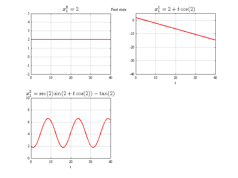
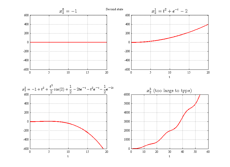
The nonlinear state space system is given by\[\begin{pmatrix} x_{1}^{\prime }\left ( t\right ) \\ x_{2}^{\prime }\left ( t\right ) \end{pmatrix} =f\left ( x,t\right ) =\begin{pmatrix} \cos x_{1}\left ( t\right ) \\ tx_{1}\left ( t\right ) +e^{-t}x_{2}\left ( t\right ) \end{pmatrix} \] With the initial conditions \[ x^{0}=\begin{pmatrix} x_{1}\left ( 0\right ) \\ x_{2}\left ( 0\right ) \end{pmatrix} =\begin{pmatrix} 2\\ -1 \end{pmatrix} \]
Let the initial guess of the solution \(x^{0}\) be the same as initial conditions 2 .
The first iteration gives \begin{align*} x^{1} & =x^{0}+{\displaystyle \int \limits _{0}^{t}} \begin{pmatrix} \cos x_{1}^{0}\\ \eta x_{1}^{0}+e^{-\eta }x_{2}^{0}\end{pmatrix} d\eta \\ & =\begin{pmatrix} 2\\ -1 \end{pmatrix} +{\displaystyle \int \limits _{0}^{t}} \begin{pmatrix} \cos 2\\ 2\eta -e^{-\eta }\end{pmatrix} d\eta \\ & =\begin{pmatrix} 2\\ -1 \end{pmatrix} +\left [ \begin{pmatrix} \eta \cos 2\\ \eta ^{2}+e^{-\eta }\end{pmatrix} \right ] _{0}^{t}\\ & =\begin{pmatrix} 2\\ -1 \end{pmatrix} +\begin{pmatrix} t\cos 2\\ t^{2}+e^{-t}-1 \end{pmatrix} \end{align*}
Therefore\[ \fbox{$x^1=\begin{pmatrix} 2+t\cos 2\\ t^{2}+e^{-t}-2 \end{pmatrix} $}\] The second iteration is\begin{align} x^{2} & =x^{0}+{\displaystyle \int \limits _{0}^{t}} \begin{pmatrix} \cos x_{1}^{1}\\ \eta x_{1}^{1}+e^{-\eta }x_{2}^{1}\end{pmatrix} d\eta \nonumber \\ & =\begin{pmatrix} 2\\ -1 \end{pmatrix} +{\displaystyle \int \limits _{0}^{t}} \begin{pmatrix} \cos \left ( 2+\eta \cos 2\right ) \\ \eta \left ( 2+\eta \cos 2\right ) +e^{-\eta }\left ( \eta ^{2}+e^{-\eta }-2\right ) \end{pmatrix} d\eta \tag{1} \end{align}
The top integral \({\displaystyle \int \limits _{0}^{t}} \cos \left ( 2+\eta \cos 2\right ) d\eta \) is evaluated using substitution. Let \(u=2+\eta \cos 2\) hence \(du=\cos 2d\eta \). When \(\eta =0,u=2\) and when \(\eta =t,u=2+t\cos 2\). Therefore the top integral becomes\begin{align}{\displaystyle \int _{0}^{t}} \cos \left ( 2+\eta \cos 2\right ) d\eta & ={\displaystyle \int _{2}^{2+t\cos 2}} \cos \left ( u\right ) \frac{du}{\cos 2}\nonumber \\ & =\frac{1}{\cos 2}{\displaystyle \int _{2}^{2+t\cos 2}} \cos \left ( u\right ) du\nonumber \\ & =\frac{1}{\cos 2}\left [ \sin \left ( u\right ) \right ] _{2}^{2+t\cos 2}\nonumber \\ & =\frac{1}{\cos 2}\left ( \sin \left ( 2+t\cos 2\right ) -\sin 2\right ) \nonumber \\ & =\sec \left ( 2\right ) \sin \left ( 2+t\cos 2\right ) -\tan 2 \tag{2} \end{align}
The lower integral in (1) is now evaluate. The first part is of this integral is\begin{align}{\displaystyle \int \limits _{0}^{t}} \eta \left ( 2+\eta \cos 2\right ) d\eta & ={\displaystyle \int \limits _{0}^{t}} \left ( 2\eta +\eta ^{2}\cos 2\right ) d\eta =\left [ \eta ^{2}+\frac{\eta ^{3}}{3}\cos 2\right ] _{0}^{t}\nonumber \\ & =t^{2}+\frac{t^{3}}{3}\cos 2 \tag{3} \end{align}
The second part is \begin{equation}{\displaystyle \int \limits _{0}^{t}} \eta ^{2}e^{-\eta }+e^{-2\eta }-2e^{-\eta }d\eta \tag{3A} \end{equation}
The first part of the above is solved using integration by parts. \(udv=uv-{\displaystyle \int } vdu\). Let \(u=\eta ^{2},dv=e^{-\eta },du=2\eta ,v=-e^{-\eta },\) therefore \begin{align*}{\displaystyle \int _{0}^{t}} \eta ^{2}e^{-\eta }d\eta & =\left [ -\eta ^{2}e^{-\eta }\right ] _{0}^{t}+{\displaystyle \int _{0}^{t}} 2\eta e^{-\eta }du\\ & =-t^{2}e^{-t}+2{\displaystyle \int _{0}^{t}} \eta e^{-\eta }du \end{align*}
The integral\({\displaystyle \int _{0}^{t}} \eta e^{-\eta }du\) is solved also by integration by parts. \(udv=uv-{\displaystyle \int } vdu\). Let \(u=\eta ,dv=e^{-\eta },du=1,v=-e^{-\eta }\), therefore\begin{align*}{\displaystyle \int _{0}^{t}} \eta ^{2}e^{-\eta }d\eta & =-t^{2}e^{-t}+2\left ( \left [ -\eta e^{-\eta }\right ] _{0}^{t}+{\displaystyle \int _{0}^{t}} e^{-\eta }du\right ) \\ & =-t^{2}e^{-t}+2\left ( -te^{-t}+\left [ -e^{-\eta }\right ] _{0}^{t}\right ) \\ & =-t^{2}e^{-t}+2\left ( -te^{-t}-e^{-t}+1\right ) \\ & =-t^{2}e^{-t}-2te^{-t}-2e^{-t}+2 \end{align*}
The remaining parts of (3A) are direct integrations that requires no special treatment, hence (3A) becomes\begin{align}{\displaystyle \int \limits _{0}^{t}} \eta ^{2}e^{-\eta }+e^{-2\eta }-2e^{-\eta }d\eta & =\left ( -t^{2}e^{-t}-2te^{-t}-2e^{-t}+2\right ) +\left [ \frac{e^{-2\eta }}{-2}\right ] _{0}^{t}+2\left [ e^{-\eta }\right ] _{0}^{t}\nonumber \\ & =\left ( -t^{2}e^{-t}-2te^{-t}-2e^{-t}+2\right ) -\frac{1}{2}\left ( e^{-2t}-1\right ) +2\left ( e^{-t}-1\right ) \nonumber \\ & =\frac{1}{2}-2te^{-t}-t^{2}e^{-t}-\frac{1}{2}e^{-2t} \tag{4} \end{align}
Putting (4),(3) and (2) into (1) gives\[ x^{2}=\begin{pmatrix} 2\\ -1 \end{pmatrix} +\begin{pmatrix} \sec \left ( 2\right ) \sin \left ( 2+t\cos 2\right ) -\tan 2\\ \frac{2}{3}t^{2}+\frac{t^{3}}{3}\cos 2+\frac{1}{2}-2te^{-t}-t^{2}e^{-t}-\frac{1}{2}e^{-2t}\end{pmatrix} \] Hence the second iteration results in\[ \fbox{$x^2=\begin{pmatrix} 2+\sec \left ( 2\right ) \sin \left ( 2+t\cos 2\right ) -\tan 2\\ -1+t^{2}+\frac{t^{3}}{3}\cos 2+\frac{1}{2}-2te^{-t}-t^{2}e^{-t}-\frac{1}{2}e^{-2t}\end{pmatrix} $}\] The third iteration \(x^{3}\) is now found using\begin{align*} x^{3} & =x^{0}+{\displaystyle \int \limits _{0}^{t}} f\left ( x^{2}\right ) d\eta \\ & =\begin{pmatrix} 2\\ -1 \end{pmatrix} +{\displaystyle \int \limits _{0}^{t}} \begin{pmatrix} \cos x_{1}^{2}\\ \eta x_{1}^{2}+e^{-\eta }x_{2}^{2}\end{pmatrix} d\eta \\ & =\begin{pmatrix} 2\\ -1 \end{pmatrix} +{\displaystyle \int \limits _{0}^{t}} \begin{pmatrix} 2+\sec \left ( 2\right ) \sin \left ( 2+\eta \cos 2\right ) -\tan 2\\ -1+\eta ^{2}+\frac{\eta ^{3}}{3}\cos 2+\frac{1}{2}-2\eta e^{-\eta }-\eta ^{2}e^{-\eta }-\frac{1}{2}e^{-2\eta }\end{pmatrix} d\eta \end{align*}
The top integral \(\left ( x_{1}^{3}\right ) \) could not be evaluated using syms. A numerical solution is needed. The lower integral which gives the second state can be evaluated directly and requires no special treatment, giving
A small function was written using syms to evaluate the Picard iterations and plot the solution. For the third iteration \(x^{3}\) the first state was not solved due to complexity of the integral. Numerical solution would be needed. The following plots show the first state and the second state.
Function to generate symbolic Picard iterations
Script to plot Picard iterations
Example using Picard iteration function Example use is
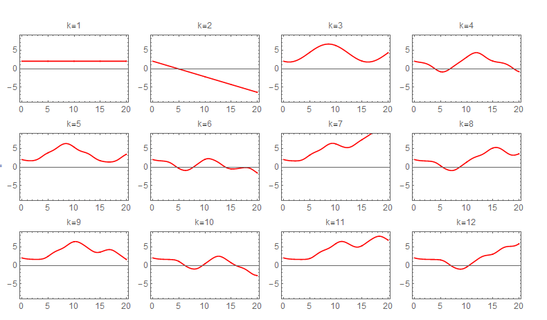
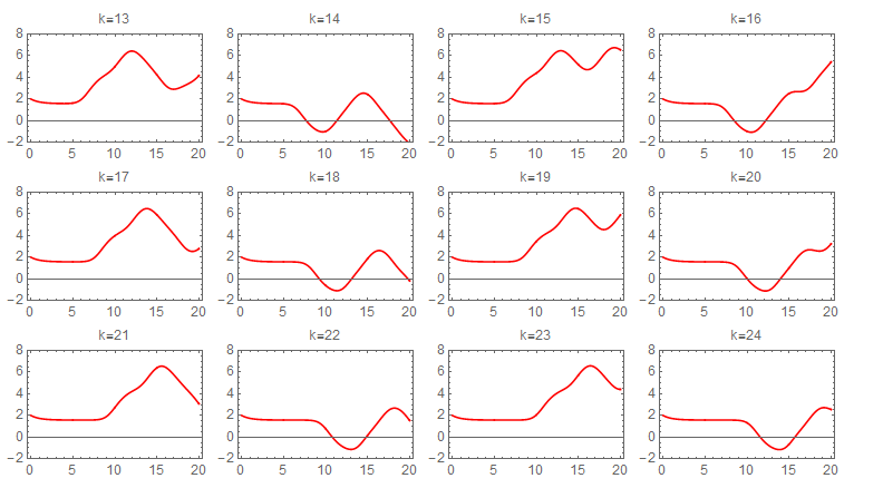
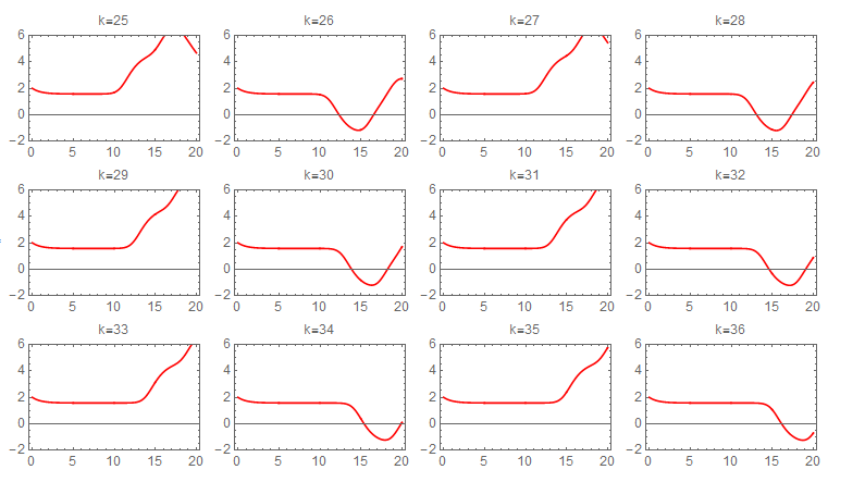
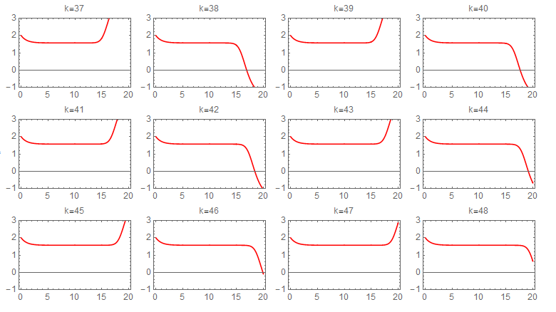
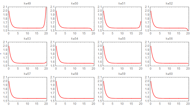
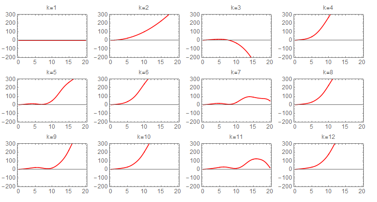
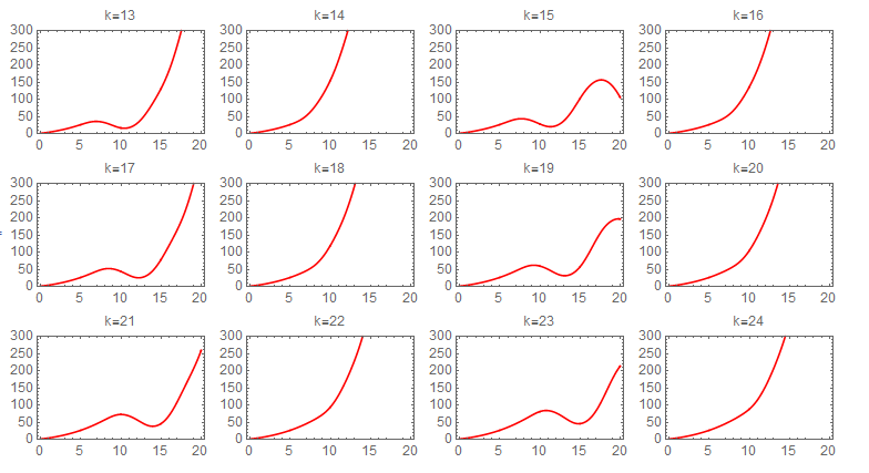
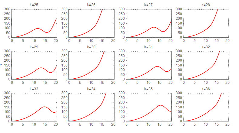
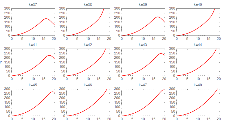
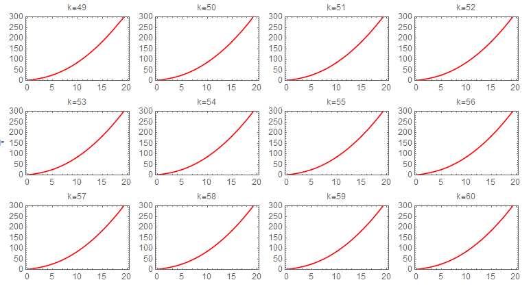
Picard iteration was integrated numerically due to difficulty of obtaining symbolic solution for each step. The following sequence of plots shows the convergence of each iteration. The first state required about 60 iterations to converge to the numerical ODE solver solution. The following shows the sequence of the iterations for the first state. Each one of these plots is 20 seconds long, and the title shows the iteration number.
second state iterations It also took about 60 Picard iterations for the second state to converge. The following is the sequence of the iterations
Since numerical integral was used, it would be useful to see what effect changing the sampling period on convergence. Three different values of \(\Delta t\) were tried. They are \((0.01,0.005,0.001)\), with units in seconds. There was no visible effect on the result. Running the program for \(80\) iterations for each case, they all converged to the same solution at the end. The following plots shows the result

Since initial guess can be any value, other than the initial conditions, it would be useful to see what effect, if any, changing the guess would have on convergence.
It was found that changing the guess to be different from initial conditions, resulted in different shape at the end of the 80 iterations. This indicates the guess used have an effect on speed of convergence. More analysis is required to inverstigate this more.
For example, this plot shows the difference at the end of 80 iterations, all using the same sampling time, with the only difference is that one used the initial conditions \([2,-1]\) as the guess, and the second used \([0,1]\) as the guess. One can see the final solution is different.

Picard iteration does converge for this non-linear system. Numerical integration was required to allow higher number of iterations to be performed, as it was not possible to do more than 3 iterations using symbolic computation.
It was found that changing the guess value from initial conditions does have an effect on convergence. But more analysis is needed to study this effect.
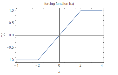
The following plot shows \(f\left ( x\right ) \)
\begin{align*} x^{1}\left ( t\right ) & =x^{0}+{\int \limits _{0}^{t}}f\left ( x^{0}\left ( \tau \right ) ,\tau \right ) d\tau \\ & =1+{\int \limits _{0}^{t}}f\left ( 1\right ) d\tau \\ & =1+{\int \limits _{0}^{t}}\frac{1}{2}d\tau \\ & =1+\frac{1}{2}t \end{align*}
Therefore \[ \fbox{$x^1\left ( t\right ) =1+\frac{1}{2}t$}\] Now for the second iteration\begin{align*} x^{\left ( 2\right ) }\left ( t\right ) & =x^{0}+{\displaystyle \int \limits _{0}^{t}} f\left ( x^{1}\left ( \tau \right ) ,\tau \right ) d\tau \\ & =x^{0}+{\displaystyle \int \limits _{0}^{t}} f\left ( 1+\frac{1}{2}\tau \right ) d\tau \end{align*}
For \(0\leq t\leq 2\) then \(f\left ( 1+\frac{1}{2}\tau \right ) =\frac{1}{2}\left ( 1+\frac{1}{2}\tau \right ) \), Therefore\begin{align*} x^{\left ( 2\right ) }\left ( t\right ) & =x^{0}+{\displaystyle \int \limits _{0}^{t}} \frac{1}{2}\left ( 1+\frac{1}{2}\tau \right ) d\tau \\ & =1+\frac{1}{2}\left [ \left ( \tau +\frac{1}{4}\tau ^{2}\right ) \right ] _{0}^{t}\\ & =1+\frac{1}{2}\left ( t+\frac{1}{4}t^{2}\right ) \\ & =\frac{t^{2}}{8}+\frac{t}{2}+1 \end{align*}
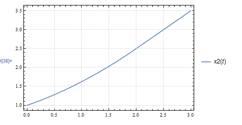
For \(t>2\), \(f\left ( t\right ) =1\), then\begin{align*} x^{\left ( 2\right ) }\left ( t\right ) & =x^{0}+{\displaystyle \int \limits _{0}^{2}} \frac{1}{2}\left ( 1+\frac{1}{2}t\right ) d\tau +{\displaystyle \int \limits _{2}^{t}} d\tau \\ & =t+\frac{1}{2} \end{align*}
Therefore\[ x^{2}\left ( t\right ) =\left \{ \begin{array} [c]{ccc}1+\frac{t}{2}+\frac{t^{2}}{8} & & t\leq 2\\ t+\frac{1}{2} & & t>2 \end{array} \right . \] A plot of \(x^{2}\left ( t\right ) \) is shown below