 ;
;
;
 ;
;
 ;
;
 ;
;
 ;
;
 ;
;
 ;
;
\[\begin{Bmatrix} \dot{x}_{1}\\ \dot{x}_{1}\end{Bmatrix} =\begin{Bmatrix} -\sin x_{2}-ax_{1}^{2}\\ \frac{-\cos x_{2}+x_{1}^{2}}{x_{1}}\end{Bmatrix} \equiv \begin{Bmatrix} f_{1}\left ( x_{1},x_{2}\right ) \\ f_{2}\left ( x_{1},x_{2}\right ) \end{Bmatrix} =\mathbf{f}\left ( x\right ) \] Letting \(a=1\), equilibrium is found by setting \(\mathbf{\dot{x}=0}\) giving\[ \mathbf{f}\left ( x_{1},x_{2}\right ) =\begin{Bmatrix} 0\\ 0 \end{Bmatrix} =\begin{Bmatrix} -\sin x_{2}-x_{1}^{2}\\ \frac{-\cos x_{2}+x_{1}^{2}}{x_{1}}\end{Bmatrix} \] The following two equations are solved for \(x_{1}\,,x_{2}\)\begin{align} -\sin x_{2}-x_{1}^{2} & =0\tag{1}\\ \frac{-\cos x_{2}+x_{1}^{2}}{x_{1}} & =0 \tag{2} \end{align}
Equation (1) gives \(x_{1}^{2}=-\sin x_{2}\). Substituting this in (2) gives\[ \frac{-\cos x_{2}-\sin x_{2}}{x_{1}}=0 \] Assuming the state \(x_{1}\) is finite, the above implies \(-\cos x_{2}-\sin x_{2}=0\) or \(\tan x_{2}=-1\) giving\[ \fbox{$x_2=\arctan \left ( -1\right ) =\frac{-\pi }{4}\pm 2n\pi $}\] For \(n=0,1,2,\cdots \) integer values . Substituting this value for \(x_{2}\) back in (1) gives\begin{align*} x_{1}^{2} & =-\sin x_{2}\\ & =-\sin \left ( \frac{-\pi }{4}\pm 2n\pi \right ) \\ & =\sin \frac{\pi }{4}\\ & =\sqrt{\frac{1}{2}} \end{align*}
Therefore\begin{align*} x_1 &=\pm \left ( \frac{1}{2} \right )^{\frac{1}{4}} \end{align*}
The equilibrium points are \(\left \{ \left ( \frac{1}{2}\right ) ^{\frac{1}{4}},\frac{-\pi }{4}\right \} \) and \(\left \{ -\left ( \frac{1}{2}\right ) ^{\frac{1}{4}},\frac{-\pi }{4}\right \} \). There are infinite number of equilibrium points for different \(n\) values but using \(n=0\) the above are the two equilibrium points considered. Approximate numerical values of the points are
\begin{align*} & \left \{ +0.8409,-0.7854\right \} \\ & \left \{ -0.8409,-0.7854\right \} \end{align*}
The point \(x^{\ast }\) was found in part(a). To verify that a point is an equilibrium point, \(\mathbf{\dot{x}}\) is evaluated at this point to see if \(\mathbf{\dot{x}=0}\). Replacing \(x_{1}\) by \(0.8409\) and \(x_{2}\) by \(-0.7854\) in\[\begin{Bmatrix} \dot{x}_{1}\\ \dot{x}_{1}\end{Bmatrix} =\begin{Bmatrix} -\sin x_{2}-x_{1}^{2}\\ \frac{-\cos x_{2}+x_{1}^{2}}{x_{1}}\end{Bmatrix} \] Gives\[\begin{Bmatrix} \dot{x}_{1}\\ \dot{x}_{1}\end{Bmatrix} =\begin{Bmatrix} 0\\ 0 \end{Bmatrix} \] Therefore \(x^{\ast }\) is an equilibrium point.
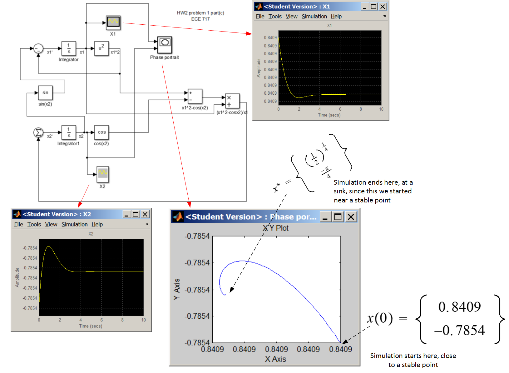
Simulink model was developed that implements part(a). Simulation was run for \(10\) seconds. The block XYgraph was used to generate phase portrait by having \(x_{1}\left ( t\right ) \) being the \(X\) input to the block and \(x_{2}\left ( t\right ) \) being the \(Y\) input to the block. Initial values of \(x_{1}\left ( 0\right ) ,x_{2}\left ( 0\right ) \) used are near \(x^{\ast }\) found above, which is \(x^{\ast }=\begin{Bmatrix} \left ( \frac{1}{2}\right ) ^{\frac{1}{4}}\\ -\frac{\pi }{4}\end{Bmatrix} \). We see that the trajectory stays near the starting point used and is a sink stable point. Increasing the simulation time has no effect, since the trajectory will move to the sink and not leave it since it is a stable sink. The following shows the model used, a plot of \(x_{1}\left ( t\right ) ,x_{2}\left ( t\right ) \) done separately, and the phase portrait plot.
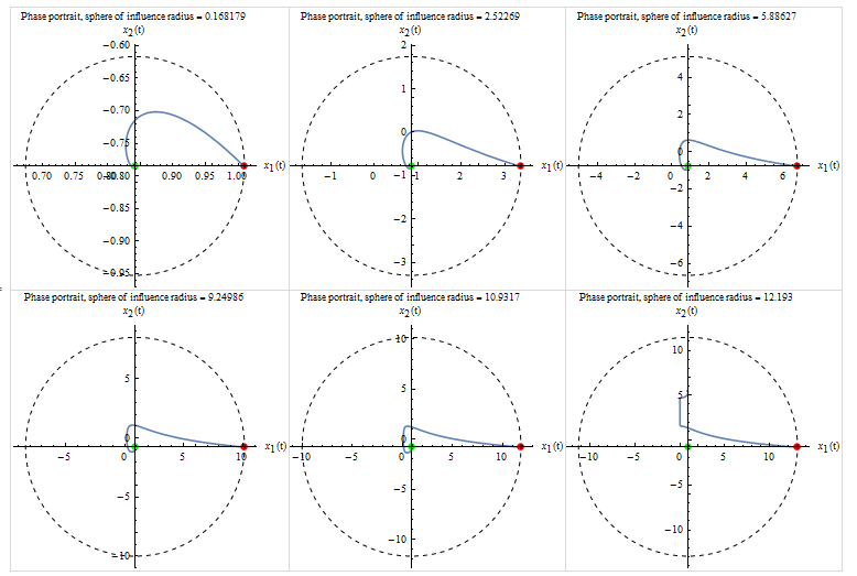
Yes, simulation indicates \(x^{\ast }\) is stable equilibrium. To estimate the circular domain of attraction, a circle centered at \(x^{\ast }\) with a radius \(r\) was used. The radius was increased in small increments. A starting initial point at the end of the radius was used to start the simulation. If the trajectory remained inside the circle and went to the sink at \(x^{\ast }\) then the radius was increased and the simulation is run again until the trajectory no longer remained inside the circle. The following are plots show this process for different values of \(r\). The result shows that the sphere of influence around \(x^{\ast }\) has radius about \(12\).
Small code written to generate the above plot
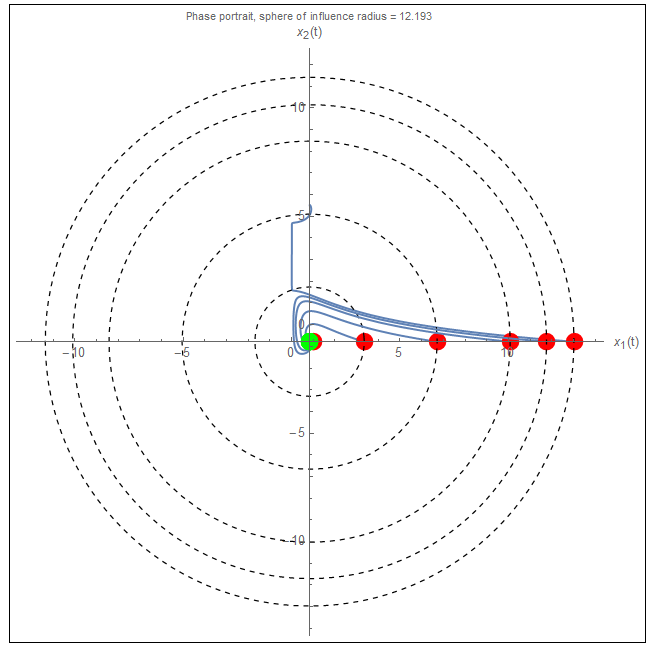
The following plot is another view of the above but displayed on the same plot
The linearized \(A\) matrix for the system, which is the Jacobian of \(f\), is now found.\begin{align*} A & =\begin{pmatrix} \frac{\partial f_{1}}{\partial x_{1}} & \frac{\partial f_{1}}{\partial x_{2}}\\ \frac{\partial f_{2}}{\partial x_{1}} & \frac{\partial f_{2}}{\partial x_{2}}\end{pmatrix} =\begin{pmatrix} \frac{\partial }{\partial x_{1}}\left ( -\sin x_{2}-ax_{1}^{2}\right ) & \frac{\partial }{\partial x_{2}}\left ( -\sin x_{2}-ax_{1}^{2}\right ) \\ \frac{\partial }{\partial x_{1}}\left ( \frac{-\cos x_{2}+x_{1}^{2}}{x_{1}}\right ) & \frac{\partial }{\partial x_{2}}\left ( \frac{-\cos x_{2}+x_{1}^{2}}{x_{1}}\right ) \end{pmatrix} \\ & =\begin{pmatrix} -2ax_{1} & -\cos x_{2}\\ \frac{1}{x_{1}^{2}}\left ( x_{1}^{2}+\cos x_{2}\right ) & \frac{1}{x_{1}}\sin x_{2}\end{pmatrix} \end{align*}
For \(a=1\)\[ A=\begin{pmatrix} -2x_{1} & -\cos x_{2}\\ 1+\frac{\cos x_{2}}{x_{1}^{2}} & \frac{1}{x_{1}}\sin x_{2}\end{pmatrix} \] The eigenvalues are found from \begin{align*} \det \left ( \lambda I-A\right ) & =0\\ p\left ( \lambda \right ) & =\begin{vmatrix} \lambda +2x_{1} & \cos x_{2}\\ -\left ( 1+\frac{\cos x_{2}}{x_{1}^{2}}\right ) & \lambda -\frac{1}{x_{1}}\sin x_{2}\end{vmatrix} \\ & =\lambda ^{2}+\lambda \left ( 2x_{1}-\frac{\sin x_{2}}{x_{1}}\right ) +\left ( \cos x_{2}-2\sin x_{2}+\cos ^{2}x_{2}\right ) \end{align*}
If the real part of each \(\lambda _{i}\) is negative, then the system is stable. The numerical values of the equilibrium points found above are substituted in \(p\left ( \lambda \right ) \) and the roots of the characteristic equation are found to determine the type of stability. For \(x_{1}=0.8409\), \(x_{2}=-0.785\,4\) the roots are\[ \fbox{$\lambda =-1.26135\pm j1.1124$} \] The system is stable since the real part of the eigenvalues is negative. The type of stability is a sink. For the second equilibrium point \(x_{1}=-0.8409\), \(x_{2}=-0.785\,4\) \(\ \)the roots are\[ \fbox{$\lambda =1.26135\pm j1.1124$} \] At this point the system is not stable since the real part is positive. The type of instability is a focus. The following is a summary of the result
| point | eigenvalues of \(A\) | stable/unstable |
| \(\left \{ x_{1}=0.8409,x_{2}=-0.785\,4\right \} \) | \(-1.26135\pm j1.1124\) | Stable, sink |
| \(\left \{ x_{1}=-0.8409,x_{2}=-0.785\,4\right \} \) | \(1.26135\pm j1.1124\) | Not stable, focus |
SOLUTION:
For the \(\frac{Y_{7}}{Y_{1}}\), There are two forward paths. The following diagrams shows them with the gain on each.

\begin{align*} F_{1} & =G_{1}G_{2}G_{3}G_{4}G_{5}\\ F_{2} & =G_{6}G_{5} \end{align*}
Now \(\Delta _{k}\) is found for each forward loop. \(\Delta _{k}\) is the Mason \(\Delta \) but with \(F_{k}\) removed from the graph. Removing \(F_{1}\) removes all the loops, hence \[ \Delta _{1}=1 \] When removing \(F_{2}\) what remains is \(L_{2}\) and \(L_{3}\), hence \begin{align*} \Delta _{2} & =1-\left ( L_{2}+L_{3}\right ) \\ & =1-\left ( -H_{2}G_{2}-H_{3}G_{3}\right ) \\ & =1+\left ( H_{2}G_{2}+H_{3}G_{3}\right ) \end{align*}
For the \(\frac{Y2}{Y_{1}}\), there is one forward path \(F_{1}=1\), the associated \(\Delta _{1}\) is\begin{align*} \Delta _{1} & =1-\sum -G_{2}H_{2}-G_{3}H_{3}-G_{4}G_{5}H_{4}-H_{6}-G_{2}G_{3}G_{4}G_{5}H_{5}\\ & +\sum \left ( -G_{2}H_{2}\right ) \left ( -G_{4}G_{5}H_{4}\right ) +\left ( -G_{2}H_{2}\right ) \left ( -H_{6}\right ) +\left ( -G_{3}H_{3}\right ) \left ( -H_{6}\right ) \\ & =1+ \overbrace{G_{2}H_{2}+G_{3}H_{3}+G_{4}G_{5}H_{4}+H_{6}+G_{2}G_{3}G_{4}G_{5}H_{5}}^{\text{one at a time}} +\overbrace{G_{2}H_{2}G_{4}G_{5}H_{4}+G_{2}H_{2}H_{6}+G_{3}H_{3}H_{6}}^{\text{two at a time}} \end{align*}
There are 8 loops. The following diagrams shows the loops with the gains

\begin{align*} \Delta &=1-\left ( L_{1}+L_{2}+L_{3}+L_{4}+L_{5}+L_{6}+L_{7}+L_{8}\right )\\ &+\left ( L_{1}L_{3}+L_{1}L_{4}+L_{1}L_{6}+L_{2}L_{4}+L_{2}L_{6} +L_{3} L_{6}+L_{3}L_{7}\right ) -L_{1}L_{3}L_{6}\\ \end{align*}
Therefore\begin{align} \Delta & =1+\overbrace{H_{1}G_{1}+H_{2}G_{2}+H_{3}G_{3}+H_{4}G_{4}G_{5}+H_{5}G_{2}G_{3}G_{4}G_{5}+H_{6}-G_{5}G_{6}H_{1}H_{5}-G_{6}G_{5}H_{4}H_{3}H_{2}H_{1}}^{\text{one at a time}} \tag{1}\\ & +\overbrace{\left ( H_{1}G_{1}H_{3}G_{3}+H_{1}G_{1}H_{4}G_{4}G_{5}+H_{1}H_{6}G_{1}+H_{2}G_{2}H_{4}G_{4}G_{5}+H_{2}G_{2}H_{6}+H_{3}G_{3}H_{6}-G_{3}H_{3}G_{6}G_{5}H_{5}H_{1}\right ) }^{\text{two at time}} \nonumber \\ & +\overbrace{H_{1}G_{1}H_{3}G_{3}H_{6}}^{\text{three at time}} \nonumber \end{align}
For \(G\left ( s\right ) =\frac{Y_{7}}{Y_{1}}\), and using result found above in part (a) and part (b)\begin{align*} G\left ( s\right ) & =\frac{Y_{7}}{Y_{1}}\\ & =\frac{\Delta _{1}F_{1}+\Delta _{2}F_{2}}{\Delta }\\ & =\frac{\left ( G_{1}G_{2}G_{3}G_{4}G_{5}\right ) +G_{6}G_{5}\left ( 1+H_{2}G_{2}+H_{3}G_{3}\right ) }{\Delta } \end{align*}
Where \(\Delta \) is given in (1) found in part(b). To obtain \(\frac{Y_{2}}{Y_{1}}\)
\begin{align*} \frac{Y_{2}}{Y_{1}} & =\frac{\Delta _1 F_1}{\Delta }\\ & =\frac{1+\overbrace{G_{2}H_{2}+G_{3} H_{3}+G_{4}G_{5}H_{4}+H_{6}+G_{2}G_{3}G_{4}G_{5}H_{5}}^{\text{one at a time}} +\overbrace{G_{2}H_{2}G_{4}G_{5}H_{4}+G_{2}H_{2}H_{6}+G_{3}H_{3}H_{6}}^{\text{two ata time}}}{\Delta }\\ & =\frac{1+G_{2}H_{2}+G_{3}H_{3}+G_{4}G_{5}H_{4}+H_{6}+G_{2}G_{3}G_{4} G_{5}H_{5}+G_{2}H_{2}G_{4}G_{5}H_{4}+G_{2}H_{2}H_{6}+G_{3}H_{3}H_{6}}{\Delta } \end{align*}
Writing \(H\left ( s\right ) \) as
\[ H\left ( s\right ) =\frac{1}{s^{2}+3s+2}\] The transfer function from \(A,B,C,D\) is\begin{align*} H_{\ast }\left ( s\right ) & =C\left ( sI-A\right ) ^{-1}B+D\\ & =\begin{pmatrix} 1 & 0 & 0 \end{pmatrix} \left ( \begin{pmatrix} s & 0 & 0\\ 0 & s & 0\\ 0 & 0 & s \end{pmatrix} -\begin{pmatrix} 1 & 1 & 0\\ 0 & -2 & 1\\ 0 & 0 & -1 \end{pmatrix} \right ) ^{-1}\begin{pmatrix} 0\\ 1\\ -2 \end{pmatrix} \\ & =\frac{1}{\left ( s-1\right ) \left ( s+2\right ) }-\frac{2}{\left ( s-1\right ) \left ( s+1\right ) \left ( s+2\right ) }\\ & =\frac{\left ( s+1\right ) -2}{\left ( s-1\right ) \left ( s+1\right ) \left ( s+2\right ) }\\ & =\frac{\left ( s-1\right ) }{\left ( s-1\right ) \left ( s+1\right ) \left ( s+2\right ) } \end{align*}
There is a zero/pole cancellation due to common factor, which results in\[ H_{\ast }\left ( s\right ) =\frac{1}{s^{2}+3s+2}\]
Hence it is a realization of \(H(s)\)
\(\left ( A,B,C,D\right ) \) is not a minimal realization of \(H\left ( s\right ) \). The actual plant given by \(H\left ( s\right ) \) is a second order. The corresponding differential equation is second order\[ y^{\prime \prime }\left ( t\right ) +3y^{\prime }\left ( t\right ) +2y\left ( t\right ) =u\left ( t\right ) \] Therefore only two states are needed. These are normally taken to be the position and the velocity (for dynamic system) \(\left ( y,y^{\prime }\right ) .\) These variables become \(x_{1},x_{2}\) in the state space formulation. However, the state space realization contains three states \(x_{1},x_{2},x_{3}\). Therefore it is not minimal.
One way to check if \(\left ( A,B,C,D\right ) \) is minimal, is to compare the eigenvalues of \(A\) to the poles of the transfer function to see if they are the same. In this case the eigenvalues of \(A\) are found from\[ \det \left ( \lambda I-A\right ) =\left \vert \begin{pmatrix} \lambda & 0 & 0\\ 0 & \lambda & 0\\ 0 & 0 & \lambda \end{pmatrix} -\begin{pmatrix} 1 & 1 & 0\\ 0 & -2 & 1\\ 0 & 0 & -1 \end{pmatrix} \right \vert =0 \] Hence solving \(\lambda ^{3}+2\lambda ^{2}-\lambda -2=0\), gives \(\lambda _{1}=-1,\lambda _{2}=1,\lambda _{3}=-2\). However the poles of \(H\left ( s\right ) \) are \(\{-1,-2\}\), therefore, since the eigenvalues of \(A\) are not the same as the poles of \(H\left ( s\right ) \) then the realization is not minimal.
Another way to verify if the system is minimal or not, is to check if the system is both controllable and observable. If one of these tests fail, then it is not a minimal realization.
Since the rank of the controllability matrix is less than the dimension of the matrix, then the realization shown is not controllable, which implies it is not minimal. No need to check for observability.
The differential equation of the system given by realization, not using the pole/zero cancellation is found from the transfer function \(\frac{\left ( s-1\right ) }{\left ( s-1\right ) \left ( s+1\right ) \left ( s+2\right ) }\) giving \[ \fbox{$y^{\prime \prime \prime }+2y^{\prime \prime }-y-2=u^{\prime }-u$} \] When the input \(u\left ( t\right ) \) is a unit step, its derivative becomes a Dirac delta \(\delta \left ( t\right ) \) which causes a short time spike at \(t=0\) causing the integrator saturation. When any input contains a derivative of unit step and higher order derivatives (doublets and triplets function), they will cause Dirac delta to show up at \(t=0\). (the time the input is applied). Therefore, the system trajectory in state space is no longer unique and hence the given state vector \(\mathbf{x}\) can not be used as state vector.
The following simulink model shows plot of the three states
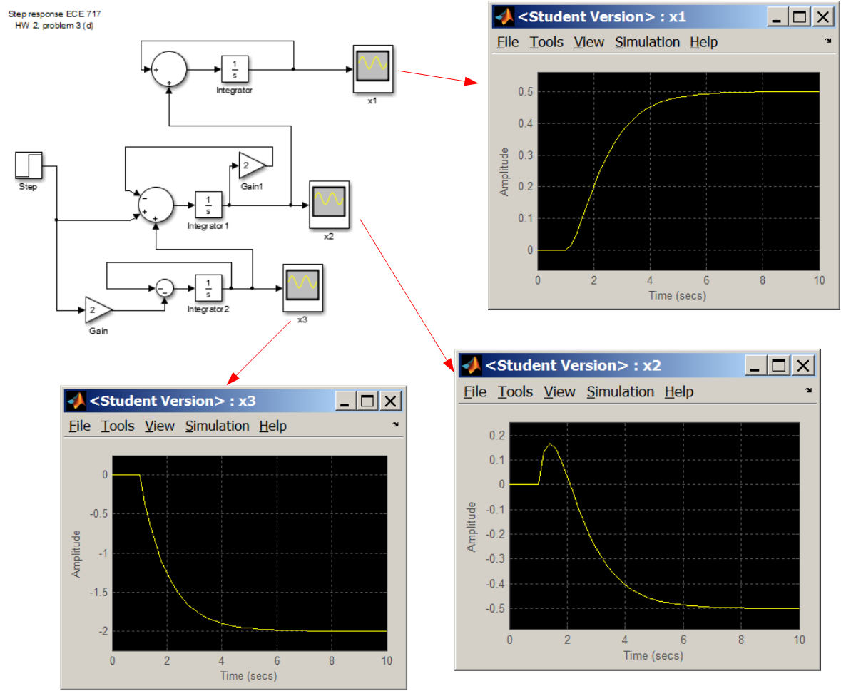
The stable response shown above can be explained as follows. Even though the derivative of the unit step causes a Dirac delta spike, its duration is very short and instantaneous and occurs at \(t=0\). Hence it did not affect the overall response shown in the plot above at steady state since the transient response have died away by then.
The system transfer function is \(H\left ( s\right ) \) of order \(r\times m~\)where \(r\) is the number of the output and \(m\) is the number of the input. Hence there are \(2\) inputs and \(3\) outputs in this example, i.e. \(D\) has size \(r\times m=3\times 2\). \[ H\left ( s\right ) =\overset{\text{number of input }\left ( m\right ) }{\overbrace{\begin{pmatrix} H_{11}\left ( s\right ) & H_{12}\left ( s\right ) \\ H_{21}\left ( s\right ) & H_{22}\left ( s\right ) \\ H_{31}\left ( s\right ) & H_{32}\left ( s\right ) \end{pmatrix} }}\] Let \[ A=\begin{pmatrix} A_{11} & 0 & 0 & 0 & 0 & 0\\ 0 & A_{12} & 0 & 0 & 0 & 0\\ 0 & 0 & A_{21} & 0 & 0 & 0\\ 0 & 0 & 0 & A_{22} & 0 & 0\\ 0 & 0 & 0 & 0 & A_{31} & 0\\ 0 & 0 & 0 & 0 & 0 & A_{32}\end{pmatrix} \] And \[ B=\begin{pmatrix} B_{11} & 0\\ 0 & B_{12}\\ B_{21} & 0\\ 0 & B_{22}\\ B_{31} & 0\\ 0 & B_{32}\end{pmatrix} \] And\[ C=\begin{pmatrix} C_{11} & C_{12} & 0 & 0 & 0 & 0\\ 0 & 0 & C_{21} & C_{22} & 0 & 0\\ 0 & 0 & 0 & 0 & C_{31} & C_{32}\end{pmatrix} \] And\[ D=\begin{pmatrix} D_{11} & D_{12}\\ D_{21} & D_{22}\\ D_{31} & D_{32}\end{pmatrix} \] Now \(H_{\ast }\left ( s\right ) =C\left ( sI-A\right ) ^{-1}B+D\) is evaluated to show it is the same as the given system transfer function.\[ \left ( sI-A\right ) ^{-1}=\begin{pmatrix} sI-A_{11} & 0 & 0 & 0 & 0 & 0\\ 0 & sI-A_{12} & 0 & 0 & 0 & 0\\ 0 & 0 & sI-A_{21} & 0 & 0 & 0\\ 0 & 0 & 0 & sI-A_{22} & 0 & 0\\ 0 & 0 & 0 & 0 & sI-A_{31} & 0\\ 0 & 0 & 0 & 0 & 0 & sI-A_{32}\end{pmatrix} ^{-1}\] This \(sI-A\) is a diagonal matrix, then its inverse is the matrix with each elements on the diagonal inverted. Hence the above becomes\[ \left ( sI-A\right ) ^{-1}=\begin{pmatrix} \left ( sI-A_{11}\right ) ^{-1} & 0 & 0 & 0 & 0 & 0\\ 0 & \left ( sI-A_{12}\right ) ^{-1} & 0 & 0 & 0 & 0\\ 0 & 0 & \left ( sI-A_{21}\right ) ^{-1} & 0 & 0 & 0\\ 0 & 0 & 0 & \left ( sI-A_{22}\right ) ^{-1} & 0 & 0\\ 0 & 0 & 0 & 0 & \left ( sI-A_{31}\right ) ^{-1} & 0\\ 0 & 0 & 0 & 0 & 0 & \left ( sI-A_{32}\right ) ^{-1}\end{pmatrix} \] Now \(C\left ( sI-A\right ) ^{-1}\) is evaluated
\begin{align*} C\left ( sI-A\right ) ^{-1} & =\begin{pmatrix} C_{11} & C_{12} & 0 & 0 & 0 & 0\\ 0 & 0 & C_{21} & C_{22} & 0 & 0\\ 0 & 0 & 0 & 0 & C_{31} & C_{32}\end{pmatrix}\begin{pmatrix} \left ( sI-A_{11}\right ) ^{-1} & 0 & 0 & 0 & 0 & 0\\ 0 & \left ( sI-A_{12}\right ) ^{-1} & 0 & 0 & 0 & 0\\ 0 & 0 & \left ( sI-A_{21}\right ) ^{-1} & 0 & 0 & 0\\ 0 & 0 & 0 & \left ( sI-A_{22}\right ) ^{-1} & 0 & 0\\ 0 & 0 & 0 & 0 & \left ( sI-A_{31}\right ) ^{-1} & 0\\ 0 & 0 & 0 & 0 & 0 & \left ( sI-A_{32}\right ) ^{-1}\end{pmatrix} \\ & =\begin{pmatrix} C_{11}\left ( sI-A_{11}\right ) ^{-1} & C_{12}\left ( sI-A_{12}\right ) ^{-1} & 0 & 0 & 0 & 0\\ 0 & 0 & C_{21}\left ( sI-A_{21}\right ) ^{-1} & C_{22}\left ( sI-A_{22}\right ) ^{-1} & 0 & 0\\ 0 & 0 & 0 & 0 & C_{31}\left ( sI-A_{31}\right ) ^{-1} & C_{32}\left ( sI-A_{32}\right ) ^{-1}\end{pmatrix} \end{align*}
Now \(C\left ( sI-A\right ) ^{-1}B\) is evaluated
\[ C\left ( sI-A\right ) ^{-1}B=\begin{pmatrix} C_{11}\left ( sI-A_{11}\right ) ^{-1} & C_{12}\left ( sI-A_{12}\right ) ^{-1} & 0 & 0 & 0 & 0\\ 0 & 0 & C_{21}\left ( sI-A_{21}\right ) ^{-1} & C_{22}\left ( sI-A_{22}\right ) ^{-1} & 0 & 0\\ 0 & 0 & 0 & 0 & C_{31}\left ( sI-A_{31}\right ) ^{-1} & C_{32}\left ( sI-A_{32}\right ) ^{-1}\end{pmatrix} \]
Which reduces to \begin{align*} C\left ( sI-A\right ) ^{-1}B & =\begin{pmatrix} B_{11} & 0\\ 0 & B_{12}\\ B_{21} & 0\\ 0 & B_{22}\\ B_{31} & 0\\ 0 & B_{32}\end{pmatrix} \\ & =\begin{pmatrix} C_{11}\left ( sI-A_{11}\right ) ^{-1}B_{11} & C_{12}\left ( sI-A_{12}\right ) ^{-1}B_{12}\\ C_{21}\left ( sI-A_{21}\right ) ^{-1}B_{21} & C_{22}\left ( sI-A_{22}\right ) ^{-1}B_{22}\\ C_{31}\left ( sI-A_{31}\right ) ^{-1}B_{31} & C_{32}\left ( sI-A_{32}\right ) ^{-1}B_{32}\end{pmatrix} \end{align*}
Finally, \(C\left ( sI-A\right ) ^{-1}B+D\) is evaluated giving\begin{align*} C\left ( sI-A\right ) ^{-1}B+D & =\begin{pmatrix} C_{11}\left ( sI-A_{11}\right ) ^{-1}B_{11} & C_{12}\left ( sI-A_{12}\right ) ^{-1}B_{12}\\ C_{21}\left ( sI-A_{21}\right ) ^{-1}B_{21} & C_{22}\left ( sI-A_{22}\right ) ^{-1}B_{22}\\ C_{31}\left ( sI-A_{31}\right ) ^{-1}B_{31} & C_{32}\left ( sI-A_{32}\right ) ^{-1}B_{32}\end{pmatrix} +\begin{pmatrix} D_{11} & D_{12}\\ D_{21} & D_{22}\\ D_{31} & D_{32}\end{pmatrix} \\ & =\begin{pmatrix} C_{11}\left ( sI-A_{11}\right ) ^{-1}B_{11}+D_{11} & C_{12}\left ( sI-A_{12}\right ) ^{-1}B_{12}+D_{12}\\ C_{21}\left ( sI-A_{21}\right ) ^{-1}B_{21}+D_{21} & C_{22}\left ( sI-A_{22}\right ) ^{-1}B_{22}+D_{22}\\ C_{31}\left ( sI-A_{31}\right ) ^{-1}B_{31}+D_{31} & C_{32}\left ( sI-A_{32}\right ) ^{-1}B_{32}+D_{32}\end{pmatrix} \end{align*}
But the above is \(\begin{pmatrix} H_{11}\left ( s\right ) & H_{12}\left ( s\right ) \\ H_{21}\left ( s\right ) & H_{22}\left ( s\right ) \\ H_{31}\left ( s\right ) & H_{32}\left ( s\right ) \end{pmatrix} \) which is what we are asked to show.
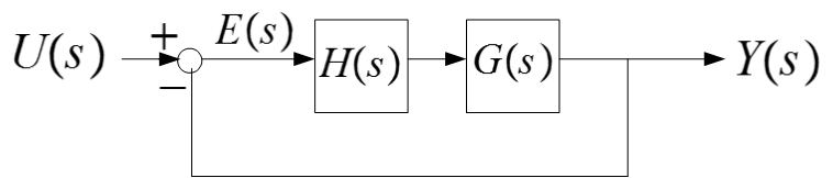
Using standard method used in SISO with attention to dimensions, one can write\begin{align*} E\left ( s\right ) & =U\left ( s\right ) -Y\left ( s\right ) \\ Y\left ( s\right ) & =E\left ( s\right ) H\left ( s\right ) G\left ( s\right ) \end{align*}
Substituting the first equation above in the second equation to eliminate \(E\left ( s\right ) \) gives (the letter \(s\) is dropped below to make the notation it more clear)\begin{align*} Y & =\left ( U-Y\right ) HG\\ & =UHG-YHG \end{align*}
Hence\[ Y+YHG=UHG \] Factoring out \(H\left ( s\right ) \) but since these are matrices, this operation generates an identity matrix with ones on the diagonal now and not scalar one as the case with SISO\[ Y\left ( I+HG\right ) =UHG \] Hence\begin{equation} \frac{Y}{U}\equiv T\left ( s\right ) =\left ( I+H\left ( s\right ) G\left ( s\right ) \right ) ^{-1}H\left ( s\right ) G\left ( s\right ) \tag{1} \end{equation} Which is what we asked to show. Another method is to use Mason rule. There is one forward path given by \(H\left ( s\right ) G\left ( s\right ) \) and one loop given by \(-H\left ( s\right ) G\left ( s\right ) \) where the negative sign is due to negative feedback, which is assumed throughout. Hence\begin{align*} \Delta & =I-\left ( -H\left ( s\right ) G\left ( s\right ) \right ) \\ & =I+H\left ( s\right ) G\left ( s\right ) \end{align*}
and \(\Delta _{1}=1\) since removing the forward path removes the loop. Hence\[ T\left ( s\right ) =\frac{\Delta _{1}\left ( H\left ( s\right ) G\left ( s\right ) \right ) }{\Delta }\] Since these are matrices, one uses matrix inversion in place of division , and the above becomes\begin{equation} \fbox{$ T\left ( s\right ) =\left ( I+H\left ( s\right ) G\left ( s\right ) \right ) ^{-1}H\left ( s\right ) G\left ( s\right )$} \tag{2} \end{equation} Which is the same as (1).
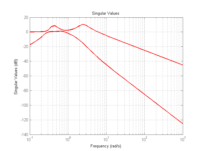
Matlab was used to plot the singular value of \(T\left ( s\right )\). The plots shows 2 lines, one for each eigenvalue, plotted from low frequency of \(0.1\) to \(10^{3}\) rad/sec. The following shows the plot and the code used
The transfer function matrix is given by \begin{align} H\left ( s\right ) & =C\left ( sI-A\right ) ^{-1}B+D\nonumber \\ & =\begin{pmatrix} 0 & 1 & -1\\ 0 & 0 & 1 \end{pmatrix} \left ( s\begin{pmatrix} 1 & 0 & 0\\ 0 & 1 & 0\\ 0 & 0 & 1 \end{pmatrix} -\begin{pmatrix} 1 & 2 & 0\\ 4 & -1 & 0\\ 0 & 0 & 1 \end{pmatrix} \right ) ^{-1}\begin{pmatrix} 1\\ 0\\ 1 \end{pmatrix} +\begin{pmatrix} 0\\ 1 \end{pmatrix} \nonumber \\ & =\begin{pmatrix} 0 & 1 & -1\\ 0 & 0 & 1 \end{pmatrix}\begin{pmatrix} s-1 & -2 & 0\\ -4 & s+1 & 0\\ 0 & 0 & s-1 \end{pmatrix} ^{-1}\begin{pmatrix} 1\\ 0\\ 1 \end{pmatrix} +\begin{pmatrix} 0\\ 1 \end{pmatrix} \tag{1} \end{align}
But \[\begin{pmatrix} s-1 & -2 & 0\\ -4 & s+1 & 0\\ 0 & 0 & s-1 \end{pmatrix} ^{-1}=\frac{adjugate\left ( A\right ) }{\det \left ( A\right ) }\] Where \begin{align*} \left \vert \left ( sI-A\right ) \right \vert & =\left ( s-1\right ) \left ( s+1\right ) \left ( s-1\right ) +2\left ( -4\left ( s-1\right ) \right ) \\ & =s^{3}-s^{2}-9s+9 \end{align*}
And adjugate of \(\left ( sI-A\right ) \) is \(cofactor\left ( sI-A\right ) ^{T}\) where\[ cofactor\left ( sI-A\right ) =\begin{pmatrix} \left ( s+1\right ) \left ( s-1\right ) & 4\left ( s-1\right ) & 0\\ 2\left ( s-1\right ) & \left ( s+1\right ) \left ( s-1\right ) & 0\\ 0 & 0 & \left ( s-1\right ) \left ( s+1\right ) -8 \end{pmatrix} \] Hence\begin{align*} adjugate\left ( sI-A\right ) & =cofactor\left ( sI-A\right ) ^{T}\\ & =\begin{pmatrix} \left ( s-1\right ) \left ( s+1\right ) & 2s-2 & 0\\ 4s-4 & \left ( s-1\right ) \left ( s+1\right ) & 0\\ 0 & 0 & \left ( s-1\right ) \left ( s+1\right ) -8 \end{pmatrix} \end{align*}
Therefore\(\allowbreak \) \[ \left ( sI-A\right ) ^{-1}=\frac{1}{s^{3}-s^{2}-9s+9}\begin{pmatrix} s^{2}-1 & 2s-2 & 0\\ 4s-4 & s^{2}-1 & 0\\ 0 & 0 & s^{2}-9 \end{pmatrix} \] And (1) now becomes\begin{align*} H\left ( s\right ) & =\frac{1}{s^{3}-s^{2}-9s+9}\begin{pmatrix} 0 & 1 & -1\\ 0 & 0 & 1 \end{pmatrix}\begin{pmatrix} s^{2}-1 & 2s-2 & 0\\ 4s-4 & s^{2}-1 & 0\\ 0 & 0 & s^{2}-9 \end{pmatrix}\begin{pmatrix} 1\\ 0\\ 1 \end{pmatrix} +\begin{pmatrix} 0\\ 1 \end{pmatrix} \\ & =\frac{1}{s^{3}-s^{2}-9s+9}\begin{pmatrix} 4s-4 & s^{2}-1 & 9-s^{2}\\ 0 & 0 & s^{2}-9 \end{pmatrix}\begin{pmatrix} 1\\ 0\\ 1 \end{pmatrix} +\begin{pmatrix} 0\\ 1 \end{pmatrix} \\ & =\frac{1}{s^{3}-s^{2}-9s+9}\begin{pmatrix} -s^{2}+4s+5\\ s^{2}-9 \end{pmatrix} +\begin{pmatrix} 0\\ 1 \end{pmatrix} \\ & =\begin{pmatrix} -\frac{-s^{2}+4s+5}{-s^{3}+s^{2}+9s-9}\\ 1-\frac{s^{2}-9}{-s^{3}+s^{2}+9s-9}\end{pmatrix} \\ & =\begin{pmatrix} \frac{-\left ( s^{2}-2s-8\right ) }{s^{3}-s^{2}-9s+9}\\ \frac{s}{s-1}\end{pmatrix} \end{align*}
Therefore \[ \fbox{$H_{11}\left ( s\right ) =\frac{-\left ( s^{2}-4s-5\right ) }{s^{3}-s^{2}-9s+9}$} \] and \[ \fbox{$H_{21}=\frac{s}{s-1}$} \]
Given the system transfer function \[ H\left ( s\right ) =\begin{pmatrix} \frac{-\left ( s^{2}-4s-5\right ) }{s^{3}-s^{2}-9s+9} & \frac{s}{s-1}\end{pmatrix} \] This new system has one output and two inputs. The system in part(a) had two outputs and one input. Let \[ A=\begin{pmatrix} A_{11} & 0\\ 0 & A_{12}\end{pmatrix} \] And \[ B=\begin{pmatrix} B_{11} & 0\\ 0 & B_{12}\end{pmatrix} \] And\[ C=\begin{pmatrix} C_{11} & C_{12}\end{pmatrix} \] And\[ D=\begin{pmatrix} D_{11} & D_{12}\end{pmatrix} \] Now \(H_{\ast }\left ( s\right ) =C\left ( sI-A\right ) ^{-1}B+D\) is evaluated giving\begin{align*} H_{\ast }\left ( s\right ) & =\begin{pmatrix} C_{11} & C_{12}\end{pmatrix}\begin{pmatrix} \left ( sI-A_{11}\right ) ^{-1} & 0\\ 0 & \left ( sI-A_{12}\right ) ^{-1}\end{pmatrix}\begin{pmatrix} B_{11} & 0\\ 0 & B_{12}\end{pmatrix} +\begin{pmatrix} D_{11} & D_{12}\end{pmatrix} \\ & =\begin{pmatrix} C_{11}\left ( sI-A_{11}\right ) ^{-1} & C_{12}\left ( sI-A_{12}\right ) ^{-1}\end{pmatrix}\begin{pmatrix} B_{11} & 0\\ 0 & B_{12}\end{pmatrix} +\begin{pmatrix} D_{11} & D_{12}\end{pmatrix} \\ & =\begin{pmatrix} C_{11}\left ( sI-A_{11}\right ) ^{-1}B_{11}+D_{11} & C_{12}\left ( sI-A_{12}\right ) ^{-1}B_{12}+D_{12}\end{pmatrix} \end{align*}
Now the following two equations are solved\begin{align*} C_{11}\left ( sI-A_{11}\right ) ^{-1}B_{11}+D_{11} & =\frac{-\left ( s^{2}-4s-5\right ) }{s^{3}-s^{2}-9s+9}\\ C_{12}\left ( sI-A_{12}\right ) ^{-1}B_{12}+D_{12} & =\frac{s}{s-1} \end{align*}
Using the companion form, the first equation above results in\begin{align*} A_{11} & =\begin{pmatrix} 0 & 1 & 0\\ 0 & 0 & 1\\ -9 & 9 & 1 \end{pmatrix} \\ B_{11} & =\begin{pmatrix} 0\\ 0\\ 1 \end{pmatrix} \\ C_{11} & =\begin{pmatrix} 5 & 4 & -1 \end{pmatrix} \\ D_{11} & =\begin{pmatrix} 0 \end{pmatrix} \end{align*}
And for the second equation \(\frac{s}{s-1}\) it is first converted to strict proper transfer function by long division, given \(1+\frac{1}{s-1}\) and now the conversion is carried out for the companion form giving\begin{align*} A_{12} & =\begin{pmatrix} 1 \end{pmatrix} \\ B_{12} & =\begin{pmatrix} 1 \end{pmatrix} \\ C_{12} & =\begin{pmatrix} 1 \end{pmatrix} \\ D_{12} & =\begin{pmatrix} 1 \end{pmatrix} \end{align*}
Therefore the realization is now found by patching the above into larger matrices as follows\[ A=\begin{pmatrix} A_{11} & 0\\ 0 & A_{12}\end{pmatrix} =\begin{pmatrix} 0 & 1 & 0 & 0\\ 0 & 0 & 1 & 0\\ -9 & 9 & 1 & 0\\ 0 & 0 & 0 & 1 \end{pmatrix} \] And \[ B=\begin{pmatrix} B_{11} & 0\\ 0 & B_{12}\end{pmatrix} =\begin{pmatrix} 0 & 0\\ 0 & 0\\ 1 & 0\\ 0 & 1 \end{pmatrix} \] And\[ C=\begin{pmatrix} C_{11} & C_{12}\end{pmatrix} =\begin{pmatrix} 5 & 4 & -1 & 1 \end{pmatrix} \] And\[ D=\begin{pmatrix} D_{11} & D_{12}\end{pmatrix} =\begin{pmatrix} 0 & 1 \end{pmatrix} \] Hence in \(x^{\prime }=Ax+Bu\) and \(y=Cx+Du\) it becomes\[ \fbox{$\begin{pmatrix} x_{1}^{\prime }\\ x_{2}^{\prime }\\ x_{3}^{\prime }\\ x_{4}^{\prime }\end{pmatrix} =\begin{pmatrix} 0 & 1 & 0 & 0\\ 0 & 0 & 1 & 0\\ -9 & 9 & 1 & 0\\ 0 & 0 & 0 & 1 \end{pmatrix}\begin{pmatrix} x_{1}\\ x_{2}\\ x_{3}\\ x_{4}\end{pmatrix} +\begin{pmatrix} 0 & 0\\ 0 & 0\\ 1 & 0\\ 0 & 1 \end{pmatrix}\begin{pmatrix} u_{1}\\ u_{2}\end{pmatrix} $}\] And\[ \fbox{$y=\begin{pmatrix} 5 & 4 & -1 & 1 \end{pmatrix}\begin{pmatrix} x_{1}\\ x_{2}\\ x_{3}\\ x_{4}\end{pmatrix} +\begin{pmatrix} 0 & 1 \end{pmatrix}\begin{pmatrix} u_{1}\\ u_{2}\end{pmatrix} $}\] is the realization.
The above is not a minimal realization. There are \(4\) states in the realization while the maximum number of poles in \(H\left ( s\right ) \) is \(3\) which is located in \(H_{11}\left ( s\right ) \). In other words, the largest part of the system is a third order differential equation, which needs only \(3\) states to fully describe. The system can be found to be not observable but it is controllable. Hence it fails one of the tests needed to qualify as a minimal realization.


