
The advection PDE in 1D is given by\[ u_{t}+au_{x}=0 \] Where \(a\) represents the speed of flow, which can be positive or negative. The Lax-Wendroff finite difference scheme for the above PDE is given by\[ u_{j}^{n+1}=u_{j}^{n}-\frac {ak}{2h}\left ( u_{j+1}^{n}-u_{j-1}^{n}\right ) +\frac {a^{2}k^{2}}{2h^{2}}\left ( u_{j-1}^{n}-2u_{j}^{n}+u_{j+1}^{n}\right ) \] where \(k\) is the time step and \(h\) is the space step. The upwind finite difference scheme for \(a>0\) is given by\[ u_{j}^{n+1}=u_{j}^{n}-\frac {ak}{h}\left ( u_{j}^{n}-u_{j-1}^{n}\right ) \] The relation between \(a,k\) and \(h\) is given by\[ courant\text { }number=\nu =\frac {ak}{h}\] Both schemes above are stable for \(\left \vert v\right \vert \leq 1\). The problem asked to use \(\nu =0.8\) and \(a=1\), giving \(k=0.8h\).
A program was written to implement these schemes for both smooth and discontinues initial conditions. The exact solution was computed from \(u=u_{0}\left ( x-at\right ) \) where \(u_{0}\left ( x\right ) \) is the initial data. \(\sin \left ( 4\pi x\right ) \) was used for smooth initial conditions.
The boundary conditions are periodic. This means that the first grid point if physically the same as the last grid point as would be the case by viewing the domain as a closed ring. The following diagram illustrates the numbering used.

Error norm calculation
The total error at a grid point \(j\) is given by \[ \mathbf {e}_{j}\mathbf {=U}_{j}\mathbf {-u}\left ( x_{j}\right ) \] Where \(\mathbf {U}_{j}\) is the numerical solution at the \(j^{th}\) grid point and \(\mathbf {u}\left ( x_{j}\right ) \) is the exact solution evaluated at the same grid point location. \(\mathbf {e}\) is a vector of length \(N\) where \(N\) is the number of grid points.
To measure the size of the error vector \(\mathbf {e}\), a grid norm is used in place of the standard vector norm. The following are the definitions of the norms used.
The result of the refinement study for smooth data for Lax-Wendroff shows that the error ratio converged to \(4\), and since the space step was divided by \(2\) at each run, this indicates a second order accuracy in time and space
The following diagram shows the results obtained. All norms gave the same order of accuracy. In the diagram below, the first ratio column represent the error ratio found using norm-2, while the second ratio column represents the norm-1 result, and the third ratio column is for the max-norm. The log plot is generated only for 2-norm. The following parameters were used: \(h=0.01,\) maximum time \(=1\) second, \(\Delta t=0.8h\), and initial conditions \(u\left ( x,0\right ) =\sin \left ( 4\pi x\right ) \) with periodic boundary conditions.

Result of refinement study for Upwind
The result of the refinement study for smooth data for upwind showed that the error ratio converged to \(2\) indicating a first order accuracy in time and space. The following diagram shows the results obtained. All norms gave the same order of accuracy.

The refinement study made in part (a) was repeated using the following initial conditions\[ u\left ( x,0\right ) =\left \{ \begin {array} [c]{cc}1 & \left \vert x-\frac {1}{2}\right \vert <\frac {1}{4}\\ 0 & otherwise \end {array} \right . \] Which is a rectangular pulse of the following shape

The following diagram shows the results obtained.
Results of refinement study for Lax-Wendroff

The following table is a summary of the results of the above refinement study for Lax-wendroff
| Norm | ratio | order of accuracy \(p=\log _{2}\left ( ratio\right ) \) |
| 1-norm | \(1.5\) | \(\frac {1}{2}\) |
| 2-norm | \(1.2\) | \(\frac {1}{4}\) |
| max-norm | \(1\) | \(0\) |
The maximum norm being zero order says that the largest error in absolute terms does not decrease. Hence for discontinues data, convergence will not occur in the max-norm, no matter how small \(h\) is made.
Results of refinement study for upwind
The following diagram shows the results obtained

The following table is a summary of the results of the above refinement study for upwind. The results are similar to Lax-Wendroff.
| Norm | ratio | order of accuracy \(p=\log _{2}\left ( ratio\right ) \) |
| 1-norm | \(1.4\) | \(0.485\) |
| 2-norm | \(1.2\) | \(\frac {1}{4}\) |
| max-norm | \(1\) | \(0\) |
It is noticed that Lax-Wendroff is more accurate scheme than upwind, but only if the initial data is smooth. For discontinuous initial conditions, Lax-wendroff loses its advantage over upwind, and both schemes gave similar order of accuracy.

Given
\[ u_{j}^{n+1}=u_{j}^{n}-C\left ( u_{j}^{n}-u_{j-1}^{n}\right ) +D\left ( u_{j+1}^{n}-u_{j}^{n}\right ) \] Writing the above in the following form\begin {align} u_{j}^{n+1} & =Cu_{j-1}^{n}+\left ( 1-\left ( C+D\right ) \right ) u_{j}^{n}+Du_{j+1}^{n}\nonumber \\ & =\begin {bmatrix} C & \left ( 1-\left ( C+D\right ) \right ) & D \end {bmatrix}\begin {bmatrix} u_{j-1}^{n}\\ u_{j}^{n}\\ u_{j+1}^{n}\end {bmatrix} \nonumber \\ & =A\ \begin {bmatrix} u_{j-1}^{n}\\ u_{j}^{n}\\ u_{j+1}^{n}\end {bmatrix} \tag {1} \end {align}
Doing the same for \(u_{j-1}^{n+1}\) results in\begin {equation} u_{j-1}^{n+1}=A\ \begin {bmatrix} u_{j-2}^{n}\\ u_{j-1}^{n}\\ u_{j}^{n}\end {bmatrix} \tag {2} \end {equation} Using the above gives\begin {align*} {\displaystyle \sum \limits _{j=-\infty }^{j=\infty }} \left \vert u_{j}^{n+1}-u_{j-1}^{n+1}\right \vert & ={\displaystyle \sum \limits _{j=-\infty }^{j=\infty }} \left \vert A\ \begin {pmatrix} u_{j-1}^{n}\\ u_{j}^{n}\\ u_{j+1}^{n}\end {pmatrix} -A\ \begin {pmatrix} u_{j-2}^{n}\\ u_{j-1}^{n}\\ u_{j}^{n}\end {pmatrix} \right \vert \\ & ={\displaystyle \sum \limits _{j=-\infty }^{j=\infty }} \left \vert A\ \begin {pmatrix} u_{j-1}^{n}-u_{j-2}^{n}\\ u_{j}^{n}-u_{j-1}^{n}\\ u_{j+1}^{n}-u_{j}^{n}\end {pmatrix} \ \right \vert \\ & ={\displaystyle \sum \limits _{j=-\infty }^{j=\infty }} \left \vert C\left ( u_{j-1}^{n}-u_{j-2}^{n}\ \right ) +\left ( 1-C-D\right ) \left ( u_{j}^{n}-u_{j-1}^{n}\right ) +D\left ( u_{j+1}^{n}-u_{j}^{n}\right ) \ \right \vert \end {align*}
Using the relation that \(\sum \left \vert A+B\right \vert \leq \sum \left ( \left \vert A\right \vert +\left \vert B\right \vert \right ) \), the above becomes\[{\displaystyle \sum \limits _{j=-\infty }^{j=\infty }} \left \vert u_{j}^{n+1}-u_{j-1}^{n+1}\right \vert \leq {\displaystyle \sum \limits _{j=-\infty }^{j=\infty }} \left \vert C\left ( u_{j-1}^{n}-u_{j-2}^{n}\right ) \right \vert +{\displaystyle \sum \limits _{j=-\infty }^{j=\infty }} \left \vert \left ( 1-C-D\right ) \left ( u_{j}^{n}-u_{j-1}^{n}\right ) \right \vert +{\displaystyle \sum \limits _{j=-\infty }^{j=\infty }} \left \vert D\left ( u_{j+1}^{n}-u_{j}^{n}\right ) \right \vert \] Given that that \(C\geq 0,D\geq 0\) and that \(\left ( 1-C-D\right ) >0\), where the last case follows from \(\left ( C+D\right ) \leq 1\), therefore \(C,D\) and \(\left ( 1-C-D\right ) \) can be taken from outside the absolute sign in the above expression leading to\[{\displaystyle \sum \limits _{j=-\infty }^{j=\infty }} \left \vert u_{j}^{n+1}-u_{j-1}^{n+1}\right \vert \leq C{\displaystyle \sum \limits _{j=-\infty }^{j=\infty }} \left \vert u_{j-1}^{n}-u_{j-2}^{n}\right \vert +\left ( 1-C-D\right ) {\displaystyle \sum \limits _{j=-\infty }^{j=\infty }} \left \vert u_{j}^{n}-u_{j-1}^{n}\right \vert +D{\displaystyle \sum \limits _{j=-\infty }^{j=\infty }} \left \vert u_{j+1}^{n}-u_{j}^{n}\right \vert \] Collecting terms with the same coefficient gives\begin {align} {\displaystyle \sum \limits _{j=-\infty }^{j=\infty }} \left \vert u_{j}^{n+1}-u_{j-1}^{n+1}\right \vert & \leq C\left ( {\displaystyle \sum \limits _{j=-\infty }^{j=\infty }} \left \vert u_{j-1}^{n}-u_{j-2}^{n}\right \vert -{\displaystyle \sum \limits _{j=-\infty }^{j=\infty }} \left \vert u_{j}^{n}-u_{j-1}^{n}\right \vert \right ) \tag {3}\\ & +D\left ( {\displaystyle \sum \limits _{j=-\infty }^{j=\infty }} \left \vert \left ( u_{j+1}^{n}-u_{j}^{n}\right ) \right \vert -{\displaystyle \sum \limits _{j=-\infty }^{j=\infty }} \left \vert \left ( u_{j}^{n}-u_{j-1}^{n}\right ) \right \vert \right ) \nonumber \\ & +{\displaystyle \sum \limits _{j=-\infty }^{j=\infty }} \left \vert \left ( u_{j}^{n}-u_{j-1}^{n}\right ) \right \vert \ \nonumber \end {align}
The first 2 expressions above in the RHS vanish, leading to the result required. To show this, Consider the first expression from the RHS above, and expanding it on the real line gives
 |
 |
Lax-Wendroff is given by\begin {align} u_{j}^{n+1} & =u_{j}^{n}-\frac {ak}{2h}\left ( u_{j+1}^{n}-u_{j-1}^{n}\right ) +\frac {a^{2}k^{2}}{2h^{2}}\left ( u_{j-1}^{n}-2u_{j}^{n}+u_{j+1}^{n}\right ) \nonumber \\ & =u_{j}^{n}\left ( 1-\frac {a^{2}k^{2}}{h^{2}}\right ) +u_{j-1}^{n}\left ( \frac {ak}{2h}+\frac {a^{2}k^{2}}{2h^{2}}\right ) +u_{j+1}^{n}\left ( \frac {a^{2}k^{2}}{2h^{2}}-\frac {ak}{2h}\right ) \tag {1} \end {align}
Eq. (1) needs to be put in the following form \(u_{j}^{n+1}=u_{j}^{n}-C\left ( u_{j}^{n}-u_{j-1}^{n}\right ) +D\left ( u_{j+1}^{n}-u_{j}^{n}\right ) \) or \begin {equation} u_{j}^{n+1}=u_{j}^{n}\left ( 1-C-D\right ) +Cu_{j-1}^{n}+Du_{j+1}^{n} \tag {2} \end {equation} Comparing Eqs. (1) and (2) leads to\begin {align} 1-C-D & =1-\frac {a^{2}k^{2}}{h^{2}}\nonumber \\ C+D & =\frac {a^{2}k^{2}}{h^{2}}\nonumber \\ C & =\frac {ak}{2h}+\frac {a^{2}k^{2}}{2h^{2}}\nonumber \\ D & =\frac {a^{2}k^{2}}{2h^{2}}-\frac {ak}{2h}=\frac {1}{2}\left ( \frac {a^{2}k^{2}}{h^{2}}-\frac {ak}{h}\right ) \tag {3} \end {align}
For the scheme to be TVD it is required that \(C\geq 0\) and \(D\geq 0\). Lax-Wendroff is stable when \(\left \vert a\right \vert \frac {k}{h}\leq 1\). Therefore this implies that \(\frac {a^{2}k^{2}}{h^{2}}<\left \vert a\right \vert \frac {k}{h}.\)Hence the constant \(D\) in Eq. (3) above will become negative. Therefore one of the conditions of TVD has been violated. Hence Lax-Wendroff is not TVD. Now consider upwind.
Consider the case \(a>0\). Upwind scheme is given by\begin {align} u_{j}^{n+1} & =u_{j}^{n}-\frac {ak}{h}\left ( u_{j}^{n}-u_{j-1}^{n}\right ) \nonumber \\ & =u_{j}^{n}\left ( 1-\frac {ak}{h}\right ) +\frac {ak}{h}u_{j-1}^{n} \tag {4} \end {align}
By comparing coefficients between Eqs. (4) and (2) results in\begin {align} 1-C-D & =1-\frac {ak}{h}\nonumber \\ C+D & =\frac {ak}{h}\nonumber \\ C & =\frac {ak}{h}\nonumber \\ D & =0 \tag {5} \end {align}
But when \(a>0\), upwind is stable when \(0\leq \frac {ak}{h}\leq 1\). Therefore \(C>0\) and all the TVD conditions above are now satisfied, Hence upwind is TVD for \(a>0\).
Now consider when \(a<0\), The upwind scheme is now given by\begin {align} u_{j}^{n+1} & =u_{j}^{n}-\frac {ak}{h}\left ( u_{j+1}^{n}-u_{j}^{n}\right ) \nonumber \\ & =u_{j}^{n}\left ( 1+\frac {ak}{h}\right ) +\left ( -\frac {ak}{h}\right ) u_{j+1}^{n} \tag {6} \end {align}
By comparing coefficients between Eqs. (6) and (2) results in\begin {align} 1-C-D & =1+\frac {ak}{h}\nonumber \\ C+D & =-\frac {ak}{h}\nonumber \\ C & =0\nonumber \\ D & =-\frac {ak}{h} \tag {5} \end {align}
since \(a<0\), then upwind is now stable when \(-1\leq \frac {ak}{h}\leq 0\). Therefore \(D>0\) in the above, and \(C+D>0\) as well, and hence all the TVD conditions are satisfied, therefore upwind is TVD for \(a<0\) as well. Therefore upwind is TVD.
Interpretation of TVD: A scheme with this property implies that the numerical solution, starting with initial data that is monotone, will remain monotone as the solution is advanced in time. This implies that no new local extrema will be created and values of local minimum are nondecreasing while values of local maximum are nonincreasing. In part (b), when initial data was discontinuous, it was observed that Lax-wendroff produced wiggles where non-existed before, meaning that new local maximum and new local minimum were created in that region. This agrees with the finding here that Lax-Wendroff is not TVD.
On the other hand, with upwind, no new wiggles were created near the discontinuity, and the numerical solution remained monotone. This agrees with the finding here that upwind is TVD scheme. A scheme which is TVD is also stable, since the TVD property will prevent any ’blow up’ in the solution due to the above properties of being TVD scheme. TVD scheme is stable, but limited to first order accuracy. To obtain more accuracy and use a second order, the price to pay is that the scheme becomes non TVD.

The PDE for linear advection equation is given by\[ u_{t}+au_{x}=0 \] The Crank Nicholson finite difference scheme for the above is\begin {equation} u_{j}^{n+1}-u_{j}^{n}+\frac {\nu }{4}\left ( u_{j+1}^{n}-u_{j-1}^{n}\right ) +\frac {\nu }{4}\left ( u_{j+1}^{n+1}-u_{j-1}^{n+1}\right ) =0 \tag {1} \end {equation} Where \(\nu =\frac {ak}{h}\), \(k\) is the time step and \(h\) is the space step. Applying Von Neumann stability analysis, let\[ u_{j}^{n+1}=g\left ( \xi \right ) e^{i\zeta x_{j}}\] and let \[ u_{j}^{n}=e^{i\zeta x_{j}}\] Substituting the above 2 equations into Eq. (1) gives\[ g\left ( \xi \right ) e^{i\zeta x_{j}}-e^{i\zeta x_{j}}+\frac {\nu }{4}\left ( e^{i\zeta x_{j}}e^{i\zeta h}-e^{i\zeta x_{j}}e^{-i\zeta h}\right ) +\frac {\nu }{4}\left ( g\left ( \xi \right ) e^{i\zeta x_{j}}e^{i\zeta h}-g\left ( \xi \right ) e^{i\zeta x_{j}}e^{-i\zeta h}\right ) =0 \] Dividing throughout by \(e^{i\zeta x_{j}}\) gives\[ g\left ( \xi \right ) -1+\frac {\nu }{4}\left ( e^{i\zeta h}-e^{-i\zeta h}\right ) +\frac {\nu }{4}g\left ( \xi \right ) \left ( e^{i\zeta h}-e^{-i\zeta h}\right ) =0 \] Solving for \(g\left ( \xi \right ) \) and applying Euler relation to convert exponential to trigonometry functions gives\begin {align*} g\left ( \xi \right ) \left ( 1+\frac {\nu i}{2}\sin \zeta h\right ) & =1-\frac {\nu i}{2}\sin \zeta h\\ g\left ( \xi \right ) & =\frac {1-\frac {\nu i}{2}\sin \zeta h}{1+\frac {\nu i}{2}\sin \zeta h} \end {align*}
Hence \[ \left \vert g\left ( \xi \right ) \right \vert ^{2}=\frac {\left \vert 1-i\frac {\nu }{2}\sin \zeta h\right \vert ^{2}}{\left \vert 1+i\frac {\nu }{2}\sin \zeta h\right \vert ^{2}}=\frac {1+\frac {\nu ^{2}}{4}\sin ^{2}\zeta h}{1+\frac {\nu ^{2}}{4}\sin ^{2}\zeta h}\] Hence \[ \left \vert g\left ( \xi \right ) \right \vert =1 \] Since \(\left \vert g\left ( \xi \right ) \right \vert \leq 1\) the scheme is unconditionally stable8.The stability of this scheme does not depend on CFL criteria, in other words, there is no dependency on \(\Delta t\) or \(h\) for the stability. In addition, it is seen that the amplitude of each Fourier mode remain constant at each time increment. High wave numbered modes as well as small wave numbered modes will remain in the numerical solution with same energy content. There is no dissipation in the numerical solution.
The following relation, which is valid due to the periodic boundary conditions being used, will be utilized in the proof below \[{\displaystyle \sum \limits _{j}} u_{j}^{n}={\displaystyle \sum \limits _{j}} u_{j-1}^{n}={\displaystyle \sum \limits _{j}} u_{j+1}^{n}\] The above relation can be more easily seen by viewing the domain as a ring, where the first grid point is physically the same as the last grid point. Therefore the location of where the sum starts is not important, since the same number of grid points will always be added as long as the sum is over the whole range. The following diagram illustrate this point.

Now, the proof will start. Starting from the C-N scheme given by\[ u_{j}^{n+1}+\frac {\nu }{4}\left ( u_{j+1}^{n+1}-u_{j-1}^{n+1}\right ) =u_{j}^{n}-\frac {\nu }{4}\left ( u_{j+1}^{n}-u_{j-1}^{n}\right ) \] And squaring each side, and summing over all \(j\) gives\[{\displaystyle \sum \limits _{j}} \left [ u_{j}^{n+1}+\frac {\nu }{4}\left ( u_{j+1}^{n+1}-u_{j-1}^{n+1}\right ) \right ] ^{2}={\displaystyle \sum \limits _{j}} \left [ u_{j}^{n}-\frac {\nu }{4}\left ( u_{j+1}^{n}-u_{j-1}^{n}\right ) \right ] ^{2}\] Expanding\begin {multline*} {\displaystyle \sum \limits _{j}} \left ( u_{j}^{n+1}\right ) ^{2}+\frac {\nu }{2}u_{j}^{n+1}\left ( u_{j+1}^{n+1}-u_{j-1}^{n+1}\right ) +\left ( \frac {\nu }{4}\right ) ^{2}\left ( u_{j+1}^{n+1}-u_{j-1}^{n+1}\right ) ^{2}=\\{\displaystyle \sum \limits _{j}} \left ( u_{j}^{n}\right ) ^{2}-\frac {\nu }{2}u_{j}^{n}\left ( u_{j+1}^{n}-u_{j-1}^{n}\right ) +\left ( \frac {\nu }{4}\right ) ^{2}\left ( u_{j+1}^{n}-u_{j-1}^{n}\right ) ^{2} \end {multline*} Moving all terms from LHS to RHS except for \({\displaystyle \sum \limits _{j}} \left ( u_{j}^{n+1}\right ) ^{2}\) the above becomes\begin {align*} {\displaystyle \sum \limits _{j}} \left ( u_{j}^{n+1}\right ) ^{2} & ={\displaystyle \sum \limits _{j}} \left ( u_{j}^{n}\right ) ^{2}-\frac {\nu }{2}\left [ u_{j}^{n}\left ( u_{j+1}^{n}-u_{j-1}^{n}\right ) +u_{j}^{n+1}\left ( u_{j+1}^{n+1}-u_{j-1}^{n+1}\right ) \right ] \\ & +\left ( \frac {\nu }{4}\right ) ^{2}\left [ \left ( u_{j+1}^{n}-u_{j-1}^{n}\right ) ^{2}-\left ( u_{j+1}^{n+1}-u_{j-1}^{n+1}\right ) ^{2}\right ] \end {align*}
Using Von Neumann, let \(u_{j}^{n+1}=\left \vert g\right \vert u_{j}^{n}\) in the above, where \(g\) is the magnification factor which was found from part (a) to be independent of \(\xi \). The above becomes\begin {align*} {\displaystyle \sum \limits _{j}} \left ( u_{j}^{n+1}\right ) ^{2} & ={\displaystyle \sum \limits _{j}} \left ( u_{j}^{n}\right ) ^{2}-\frac {\nu }{2}\left [ u_{j}^{n}\left ( u_{j+1}^{n}-u_{j-1}^{n}\right ) +\left \vert g\right \vert ^{2}u_{j}^{n}\left ( u_{j+1}^{n}-u_{j-1}^{n}\right ) \right ] \\ & +\left ( \frac {\nu }{4}\right ) ^{2}\left [ \left ( u_{j+1}^{n}-u_{j-1}^{n}\right ) ^{2}-\left \vert g\right \vert ^{2}\left ( u_{j+1}^{n}-u_{j-1}^{n}\right ) ^{2}\right ] \end {align*}
Since \(\left \vert g\right \vert =1\) as was found in part(a), then the last term in the RHS above will vanish resulting in\begin {align} {\displaystyle \sum \limits _{j}} \left ( u_{j}^{n+1}\right ) ^{2} & ={\displaystyle \sum \limits _{j}} \left ( u_{j}^{n}\right ) ^{2}-\frac {\nu }{2}\left [ u_{j}^{n}\left ( u_{j+1}^{n}-u_{j-1}^{n}\right ) +u_{j}^{n}\left ( u_{j+1}^{n}-u_{j-1}^{n}\right ) \right ] \nonumber \\ & ={\displaystyle \sum \limits _{j}} \left ( u_{j}^{n}\right ) ^{2}-\nu \ u_{j}^{n}\left ( u_{j+1}^{n}-u_{j-1}^{n}\right ) \nonumber \\ & ={\displaystyle \sum \limits _{j}} \left ( u_{j}^{n}\right ) ^{2}+\nu \ \left ( {\displaystyle \sum \limits _{j}} u_{j}^{n}u_{j-1}^{n}-{\displaystyle \sum \limits _{j}} u_{j}^{n}u_{j+1}^{n}\right ) \tag {1} \end {align}
Due to the periodic boundary9 conditions \({\displaystyle \sum \limits _{j}} u_{j}^{n}u_{j-1}^{n}={\displaystyle \sum \limits _{j}} u_{j}^{n}u_{j+1}^{n}\), Therefore Eq. (1) reduces to
\begin {equation} {\displaystyle \sum \limits _{j}} \left ( u_{j}^{n+1}\right ) ^{2}={\displaystyle \sum \limits _{j}} \left ( u_{j}^{n}\right ) ^{2} \tag {2} \end {equation} But by definition
\[ \left \Vert u\right \Vert _{2}^{2}={\displaystyle \sum \limits _{j}} u^{2}\] Hence Eq. (2) can be written as\begin {equation} \left \Vert u^{n+1}\right \Vert _{2}^{2}=\left \Vert u^{n}\right \Vert _{2}^{2}\nonumber \end {equation} or\begin {equation} \left \Vert u^{n+1}\right \Vert _{2}=\left \Vert u^{n}\right \Vert _{2} \tag {3} \end {equation} Similarly \(\left \Vert u^{n}\right \Vert _{2}=\left \Vert u^{n-1}\right \Vert _{2}=\cdots =\left \Vert u^{0}\right \Vert _{2}\), therefore Eq. (3) becomes\[ \left \Vert u^{n+1}\right \Vert _{2}=\left \Vert u^{0}\right \Vert _{2}\]
The C-N scheme was implemented for the 1D advection PDE. The source code is shown in the appendix. The following diagram shows the result for the initial conditions as given in part (b). The result for C-N is shown next to the solution produced by Lax-Wendroff in order to compare the results
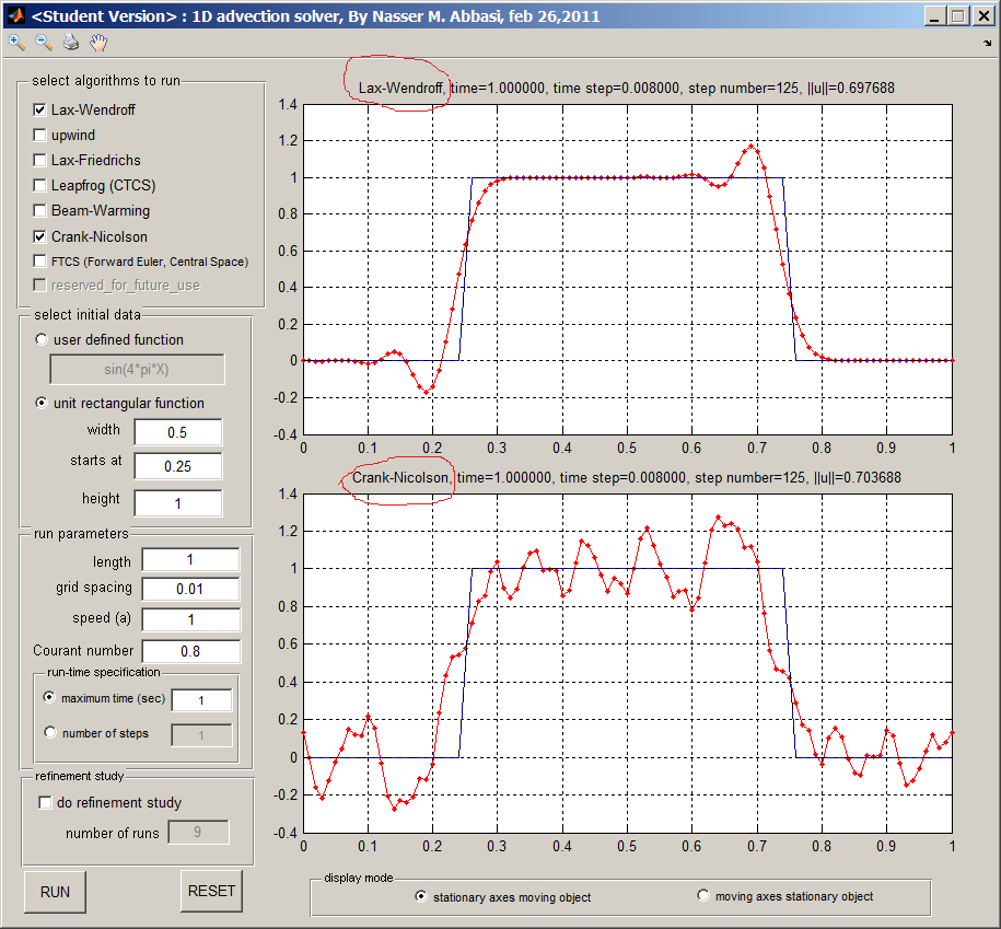
C-N shows more wiggles near the boundaries than Lax-Wendroff. Both are not TVD schemes, so starting with non-smooth initial data, it was expected to see wiggles in both cases.
C-N scheme showed more wiggles and they appeared earlier in time as well, even though the solution was stable all the time, since these did not grow when the running time was made longer (It was shown in part(a) that the scheme is unconditionally stable). Norm-2 of the solution was displayed all the time and it remained the same value through the run-time, even as wiggles appeared in the solution. This was the case for both schemes shown.
This result shows that 2-norm of the numerical solution is stable as the 2-norm of the numerical solution did not grow with time. The scheme is non-dissipative at all, and high frequency modes did not attenuate, leading the solution observed. Using such non-dissipative schemes on non-smooth data does not appear to be a good idea. The following diagram below is another illustration to compare Lax-Wendroff with C-N with \(h=0.005\), showing the numerical solution at \(t=0.04\) seconds.

The top diagram shows Lax-Wendroff, and the bottom one shows C-N. Notice that wiggles are larger in amplitude for C-N since its magnification factor is constant at \(1\), resulting in no attenuation at all in the large spatial frequency present in the initial data.
8May be we should call this as marginally stable? Since there is no attenuation and also there is no magnification.
9Side note: Initially I thought I might have to use the Schawrz inequality \(\left \vert u\cdot v\right \vert \leq \left \Vert u\right \Vert \left \Vert v\right \Vert \), to write
\[{\displaystyle \sum \limits _{j}} u_{j}^{n}u_{j+1}^{n}\leq \sqrt {{\displaystyle \sum \limits _{j}} \left ( u_{j}^{n}\right ) ^{2}}\sqrt {{\displaystyle \sum \limits _{j}} \left ( u_{j+1}^{n}\right ) ^{2}}\]
And due to periodic boundary conditions, obtain \({\displaystyle \sum \limits _{j}} \left ( u_{j}^{n}\right ) ^{2}={\displaystyle \sum \limits _{j}} \left ( u_{j+1}^{n}\right ) ^{2}\), and so \({\displaystyle \sum \limits _{j}} u_{j}^{n}u_{j+1}^{n}\leq {\displaystyle \sum \limits _{j}} \left ( u_{j}^{n}\right ) ^{2}\) But this turned out not to be required.