Solve number of mechanical problems, generate velocity, acceleration and force diagrams, and the equations of motions. Add solution using Lagrangian as well. 5 problems

Solve number of mechanical problems, generate velocity, acceleration and force diagrams, and the equations of motions. Add solution using Lagrangian as well. 5 problems
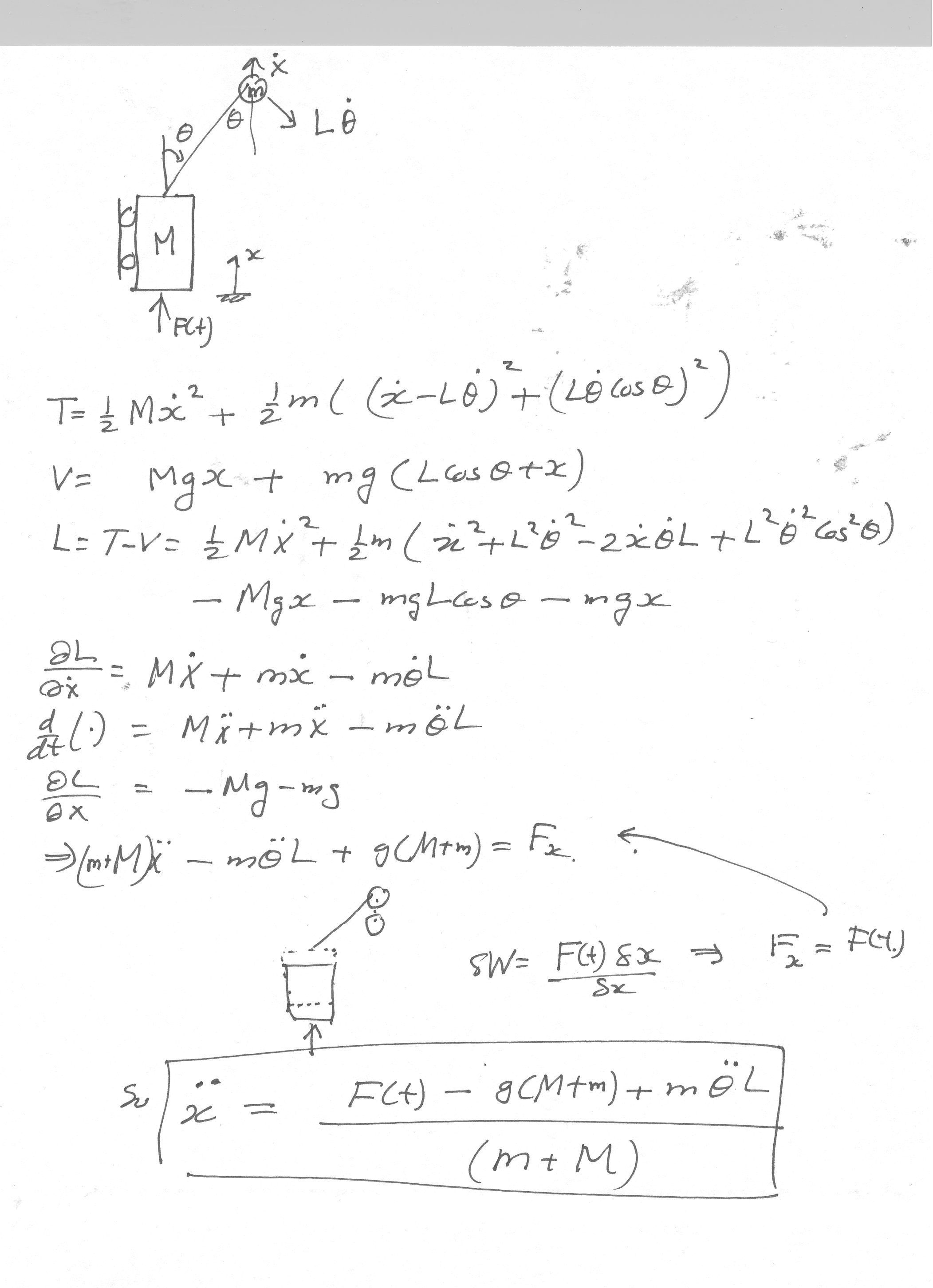
Generalized coordinates are: \(x,\theta \)


There are 4 unknowns in the system, \(H,V,x^{\prime \prime },\theta ^{\prime \prime }\). Therefore, we need 4 equations.
Starting with equation of motion for mass \(M\) \begin{align*} \overrightarrow{\sum }F_x &= Mx'' \\ F(t) -kx -H &= Mx'' \tag{1} \end{align*}
For mass \(m\)

\begin{align*} \overrightarrow{\sum }F_{x} &= m\left ( x''+L\theta '' \cos \theta -L(\theta ')^2 \sin \theta \right ) \\ H &= m\left (x'' + L\theta '' \cos \theta - L(\theta ')^2 \sin \theta \right ) \tag{2} \end{align*}
\begin{align*} \uparrow \sum F_{y} &= m\left ( -L\theta '' \sin \theta - L(\theta ')^2\cos \theta \right ) \\ V-mg &= - m\left ( L\theta '' \sin \theta +L(\theta ')^2\cos \theta \right ) \tag{3} \end{align*}
Take moments around mass \(m\), anti-clockwise is positive, hence\begin{align*} HL\cos \theta -VL\sin \theta & =0\\ V & =H\frac{\cos \theta }{\sin \theta } \end{align*}
Substituting the above in (3) gives\[ H\frac{\cos \theta }{\sin \theta }-mg=-m\left ( L\theta ^{\prime \prime }\sin \theta +L\left ( \theta ^{\prime }\right ) ^{2}\cos \theta \right ) \] Now, substituting \(H\) from (2) into the above gives\begin{align*} \frac{m\left ( x^{\prime \prime }+L\theta ^{\prime \prime }\cos \theta -L\left ( \theta ^{\prime }\right ) ^{2}\sin \theta \right ) \cos \theta }{\sin \theta }-mg & =-m\left ( L\theta ^{\prime \prime }\sin \theta +L\left ( \theta ^{\prime }\right ) ^{2}\cos \theta \right ) \\ \left ( x^{\prime \prime }+L\theta ^{\prime \prime }\cos \theta -L\left ( \theta ^{\prime }\right ) ^{2}\sin \theta \right ) \cos \theta -g\sin \theta & =-L\theta ^{\prime \prime }\sin ^{2}\theta -L\left ( \theta ^{\prime }\right ) ^{2}\cos \theta \sin \theta \\ L\theta ^{\prime \prime }\cos ^{2}\theta +L\theta ^{\prime \prime }\sin ^{2}\theta & =g\sin \theta -x^{\prime \prime }\cos \theta \\ \theta ^{\prime \prime } & =\frac{g\sin \theta -x^{\prime \prime }\cos \theta }{L} \end{align*}
Now, substituting \(H\) into (1) gives\begin{align*} F\left ( t\right ) -kx-H & =Mx^{\prime \prime }\\ F\left ( t\right ) -kx-m\left ( x^{\prime \prime }+L\theta ^{\prime \prime }\cos \theta -L\left ( \theta ^{\prime }\right ) ^{2}\sin \theta \right ) & =Mx^{\prime \prime }\\ x^{\prime \prime }\left ( M+m\right ) & =F\left ( t\right ) -kx-mL\theta ^{\prime \prime }\cos \theta +mL\left ( \theta ^{\prime }\right ) ^{2}\sin \theta \\ x^{\prime \prime } & =\frac{F\left ( t\right ) -kx-mL\theta ^{\prime \prime }\cos \theta +mL\left ( \theta ^{\prime }\right ) ^{2}\sin \theta }{M+m} \end{align*}
\begin{align} x^{\prime \prime } & =\frac{F\left ( t\right ) -kx-mL\theta ^{\prime \prime }\cos \theta +mL\left ( \theta ^{\prime }\right ) ^{2}\sin \theta }{M+m}\tag{4}\\ \theta ^{\prime \prime } & =\frac{g\sin \theta -x^{\prime \prime }\cos \theta }{L} \tag{5} \end{align}
Substitute Eq. (5) into Eq. (4) gives\begin{align} x^{\prime \prime } & =\frac{F\left ( t\right ) -kx-mL\left [ \frac{g\sin \theta -x^{\prime \prime }\cos \theta }{L}\right ] \cos \theta +mL\left ( \theta ^{\prime }\right ) ^{2}\sin \theta }{M+m}\nonumber \\ & =\frac{F\left ( t\right ) -kx-mg\sin \theta \cos \theta +mx^{\prime \prime }\cos ^{2}\theta +mL\left ( \theta ^{\prime }\right ) ^{2}\sin \theta }{M+m}\nonumber \\ x^{\prime \prime }\left ( M+m\right ) -mx^{\prime \prime }\cos ^{2}\theta & =F\left ( t\right ) -kx-mg\sin \theta \cos \theta +mL\left ( \theta ^{\prime }\right ) ^{2}\sin \theta \nonumber \\ x^{\prime \prime } & =\frac{F\left ( t\right ) -kx-mg\sin \theta \cos \theta +mL\left ( \theta ^{\prime }\right ) ^{2}\sin \theta }{\left ( M+m-m\cos ^{2}\theta \right ) } \tag{4A} \end{align}
Also, we can solve for \(\theta ^{\prime \prime }\) by Substituting Eq. (4) into (5)\begin{align} \theta ^{\prime \prime } & =\frac{g\sin \theta -\left ( \frac{F\left ( t\right ) -kx-mL\theta ^{\prime \prime }\cos \theta +mL\left ( \theta ^{\prime }\right ) ^{2}\sin \theta }{M+m}\right ) \cos \theta }{L}\nonumber \\ L\theta ^{\prime \prime }\left ( M+m\right ) & =g\sin \theta \left ( M+m\right ) -\left ( F\left ( t\right ) -kx-mL\theta ^{\prime \prime }\cos \theta +mL\left ( \theta ^{\prime }\right ) ^{2}\sin \theta \right ) \cos \theta \nonumber \\ L\theta ^{\prime \prime }\left ( M+m\right ) & =g\sin \theta \left ( M+m\right ) -F\left ( t\right ) \cos \theta +kx\cos \theta +mL\theta ^{\prime \prime }\cos ^{2}\theta -mL\left ( \theta ^{\prime }\right ) ^{2}\sin \theta \cos \theta \nonumber \\ L\theta ^{\prime \prime }\left ( M+m\right ) -mL\theta ^{\prime \prime }\cos ^{2}\theta & =g\sin \theta \left ( M+m\right ) -F\left ( t\right ) \cos \theta +kx\cos \theta -mL\left ( \theta ^{\prime }\right ) ^{2}\sin \theta \cos \theta \nonumber \\ \theta ^{\prime \prime } & =\frac{g\sin \theta \left ( M+m\right ) -F\left ( t\right ) \cos \theta +kx\cos \theta -mL\left ( \theta ^{\prime }\right ) ^{2}\sin \theta \cos \theta }{L\left ( M+m-m\cos ^{2}\theta \right ) } \tag{5A} \end{align}
Eqs. (4A) and (5A) is what will be used to convert the system to state space since they are in decoupled form.
Using the decoupled ODE’s above, Eqs (4A) and (5A), and introducing 4 state variables \(x_{1},x_{2},x_{3}x_{4}\) we obtain\begin{align*} \begin{pmatrix} x_{1}\\ x_{2}\\ x_{3}\\ x_{4}\end{pmatrix} & =\begin{pmatrix} x\\ \theta \\ x^{\prime }\\ \theta ^{\prime }\end{pmatrix} \overset{\frac{d}{dt}}{\rightarrow }\begin{pmatrix} \dot{x}_{1}\\ \dot{x}_{2}\\ \dot{x}_{3}\\ \dot{x}_{4}\end{pmatrix} =\begin{pmatrix} x^{\prime }\\ \theta ^{\prime }\\ x^{\prime \prime }\\ \theta ^{\prime \prime }\end{pmatrix} \\\begin{pmatrix} \dot{x}_{1}\\ \dot{x}_{2}\\ \dot{x}_{3}\\ \dot{x}_{4}\end{pmatrix} & =\begin{pmatrix} x_{3}\\ x_{4}\\ \frac{F\left ( t\right ) -kx-mg\sin \theta \cos \theta +mL\left ( \theta ^{\prime }\right ) ^{2}\sin \theta }{\left ( M+m-m\cos ^{2}\theta \right ) }\\ \frac{g\sin \theta \left ( M+m\right ) -F\left ( t\right ) \cos \theta +kx\cos \theta -mL\left ( \theta ^{\prime }\right ) ^{2}\sin \theta \cos \theta }{L\left ( M+m-m\cos ^{2}\theta \right ) }\end{pmatrix} \\\begin{pmatrix} \dot{x}_{1}\\ \dot{x}_{2}\\ \dot{x}_{3}\\ \dot{x}_{4}\end{pmatrix} & =\begin{pmatrix} x_{3}\\ x_{4}\\ \frac{F\left ( t\right ) -kx_{1}-mg\sin x_{2}\cos x_{2}+mLx_{4}^{2}\sin x_{1}}{\left ( M+m-m\cos ^{2}x_{2}\right ) }\\ \frac{g\sin x_{2}\left ( M+m\right ) -F\left ( t\right ) \cos x_{2}+kx_{1}\cos x_{2}-mLx_{4}^{2}\sin x_{2}\cos x_{2}}{L\left ( M+m-m\cos ^{2}x_{2}\right ) }\end{pmatrix} \end{align*}
To verify the solution above, try using Lagrangian method. Let \(L\) be the Lagrangian, and let \(T\) be the kinetic energy of the system, and \(U\) the potential energy.\[ L=T-U \] \[ T=\frac{1}{2}M\dot{x}^{2}+\frac{1}{2}mv^{2}\] Where \(v\) is the speed of the mass \(m\) which is

\begin{align*} v^{2} & =\left ( \dot{x}+v_{x}\right ) ^{2}+v_{y}^{2}\\ & =\left ( \dot{x}+v\cos \theta \right ) ^{2}+\left ( v\sin \theta \right ) ^{2}\\ & =\left ( \dot{x}+L\dot{\theta }\cos \theta \right ) ^{2}+\left ( L\dot{\theta }\sin \theta \right ) ^{2}\\ & =\dot{x}^{2}+\left ( L\dot{\theta }\right ) ^{2}\cos ^{2}\theta +2\dot{x}L\dot{\theta }\cos \theta +\left ( L\dot{\theta }\right ) ^{2}\sin ^{2}\theta \\ & =\dot{x}^{2}+\left ( L\dot{\theta }\right ) ^{2}+2\dot{x}L\dot{\theta }\cos \theta \end{align*}
Hence\[ T=\frac{1}{2}M\dot{x}^{2}+\frac{1}{2}m\left ( \dot{x}^{2}+\left ( L\dot{\theta }\right ) ^{2}+2\dot{x}L\dot{\theta }\cos \theta \right ) \] For the potential energy, the mass \(M\) has\[ U_{M}=\frac{1}{2}kx^{2}\] and the mass \(m\) is losing PE, hence, assuming that the zero potential energy is at the ground level\[ U_{m}=mgL\cos \theta \] Therefore, \(L\) becomes\[ L=\frac{1}{2}M\dot{x}^{2}+\frac{1}{2}m\left ( \dot{x}^{2}+\left ( L\dot{\theta }\right ) ^{2}+2\dot{x}L\dot{\theta }\cos \theta \right ) -\left ( \frac{1}{2}kx^{2}+mgL\cos \theta \right ) \] To obtain equations of motion, evaluate \begin{equation} \frac{d}{dt}\left ( \frac{\partial L}{\partial \dot{x}}\right ) -\frac{\partial L}{\partial x}=F \tag{1} \end{equation} and\begin{equation} \frac{d}{dt}\left ( \frac{\partial L}{\partial \dot{\theta }}\right ) -\frac{\partial L}{\partial \theta }=0 \tag{2} \end{equation} For \(M\) we obtain\[ \frac{\partial L}{\partial \dot{x}}=M\dot{x}+m\dot{x}+mL\dot{\theta }\cos \theta \]
\[ \frac{d}{dt}\left ( \frac{\partial L}{\partial \dot{x}}\right ) =M\ddot{x}+m\ddot{x}+mL\ddot{\theta }\cos \theta -mL\dot{\theta }^{2}\sin \theta \]
\[ \frac{\partial L}{\partial x}=-kx \] Hence, for the mass \(M\), the equation of motion is\begin{align} M\ddot{x}+m\ddot{x}+mL\ddot{\theta }\cos \theta -mL\dot{\theta }^{2}\sin \theta +kx & =F\nonumber \\ \ddot{x} & =\frac{F-mL\ddot{\theta }\cos \theta +mL\dot{\theta }^{2}\sin \theta -kx}{M+m} \tag{4C} \end{align}
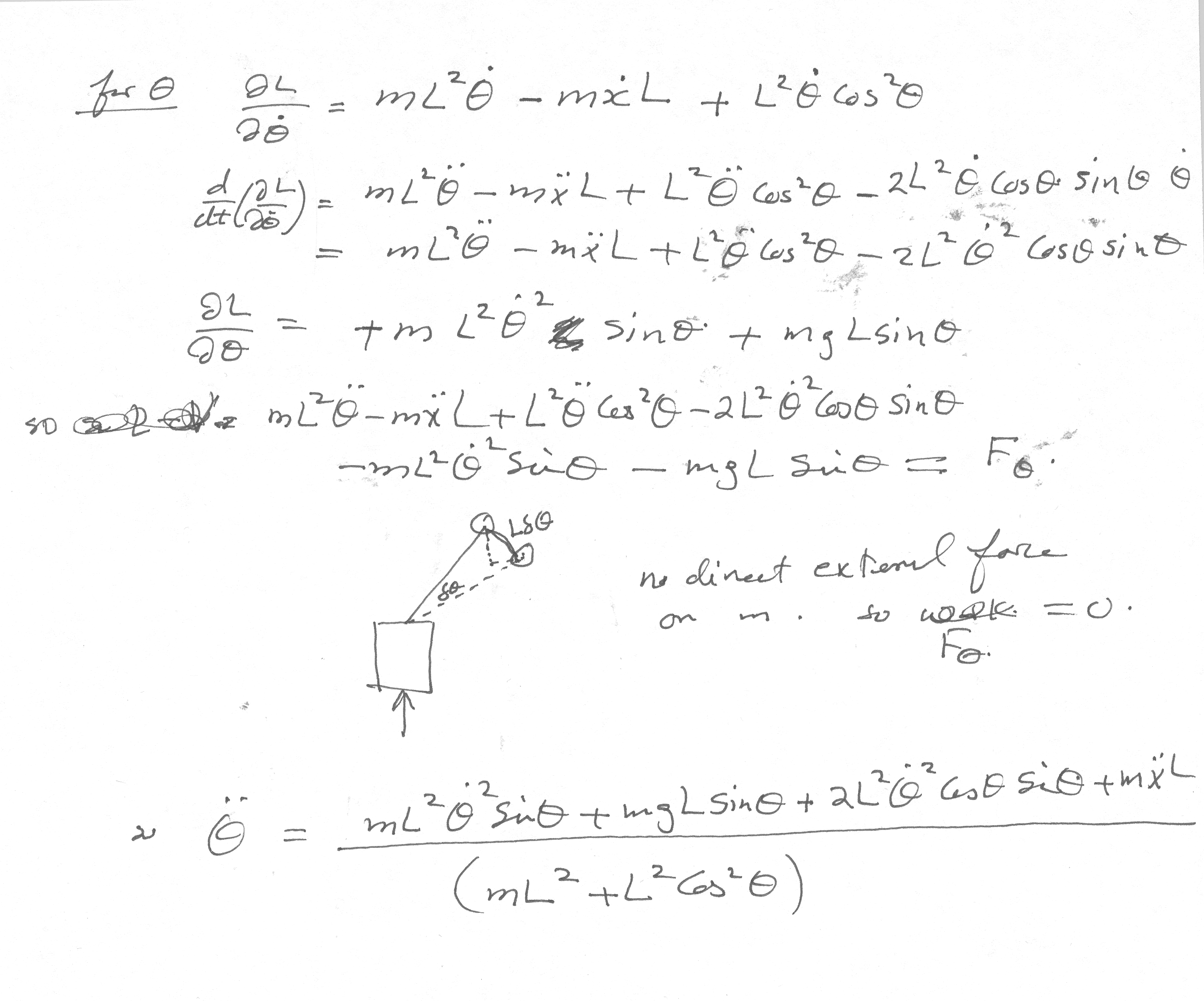
To find EQM for mass \(m\), evaluate \(\frac{d}{dt}\left ( \frac{\partial L}{\partial \dot{\theta }}\right ) -\frac{\partial L}{\partial \theta }=0\)
\[ \frac{\partial L}{\partial \dot{\theta }}=mL^{2}\dot{\theta }+m\dot{x}L\cos \theta \]
\[ \frac{d}{dt}\left ( \frac{\partial L}{\partial \dot{\theta }}\right ) =mL^{2}\ddot{\theta }+m\ddot{x}L\cos \theta -m\dot{x}L\dot{\theta }\sin \theta \]
\[ \frac{\partial L}{\partial \theta }=-m\dot{x}L\dot{\theta }\sin \theta +mgL\sin \theta \] Hence EQM is\begin{align} \frac{d}{dt}\left ( \frac{\partial L}{\partial \dot{\theta }}\right ) -\frac{\partial L}{\partial \theta } & =0\nonumber \\ mL^{2}\ddot{\theta }+m\ddot{x}L\cos \theta -m\dot{x}L\dot{\theta }\sin \theta -\left ( -m\dot{x}L\dot{\theta }\sin \theta +mgL\sin \theta \right ) & =0\nonumber \\ L\ddot{\theta }+\ddot{x}\cos \theta -\dot{x}\dot{\theta }\sin \theta +\dot{x}\dot{\theta }\sin \theta -g\sin \theta & =0\nonumber \\ L\ddot{\theta }+\ddot{x}\cos \theta -g\sin \theta & =0\nonumber \\ \ddot{\theta } & =\frac{g\sin \theta -\ddot{x}\cos \theta }{L} \tag{5C} \end{align}
Comparing Eqs. 4,5 to Eqs. 4C,5C, we see they are the same.
Generalized coordinates are: \(x,\theta \)


There are 4 unknowns in the system, \(H,V,x'',\theta ''\). Therefore, we need 4 equations.
Starting with equation of motion for mass \(M\)\begin{align} \overrightarrow{\sum }F_{x} & =Mx^{\prime \prime }\nonumber \\ F\left ( t\right ) -kx-H & =Mx^{\prime \prime } \tag{1} \end{align}
For rod

\begin{align} \overrightarrow{\sum }F_{x} & =m\left ( x^{\prime \prime }+a\theta ^{\prime \prime }\cos \theta -a\left ( \theta ^{\prime }\right ) ^{2}\sin \theta \right ) \nonumber \\ H & =m\left ( x^{\prime \prime }+a\theta ^{\prime \prime }\cos \theta -a\left ( \theta ^{\prime }\right ) ^{2}\sin \theta \right ) \tag{2} \end{align}
\begin{align} \overrightarrow{\sum }F_{y}&=m\left ( -a\theta ^{\prime \prime }\sin \theta -a\left ( \theta ^{\prime }\right ) ^{2}\cos \theta \right ) \nonumber \\ V-mg & =-m\left ( a\theta ^{\prime \prime }\sin \theta +a\left ( \theta ^{\prime }\right ) ^{2}\cos \theta \right ) \tag{3} \end{align}
Take moments around c.g., anti-clockwise is positive, hence\begin{align*} Ha\cos \theta -Va\sin \theta & =-I_{g}\theta ^{\prime \prime }\\ V & =\frac{Ha\cos \theta +I_{g}\theta ^{\prime \prime }}{a\sin \theta } \end{align*}
Substituting the above in (3) gives\begin{align*} \frac{Ha\cos \theta +I_{g}\theta ^{\prime \prime }}{a\sin \theta }-mg & =-m\left ( a\theta ^{\prime \prime }\sin \theta +a\left ( \theta ^{\prime }\right ) ^{2}\cos \theta \right ) \\ H & =\frac{\left [ -m\left ( a\theta ^{\prime \prime }\sin \theta +a\left ( \theta ^{\prime }\right ) ^{2}\cos \theta \right ) +mg\right ] a\sin \theta -I_{g}\theta ^{\prime \prime }}{a\cos \theta } \end{align*}
Substituting \(H\) from (2) into the above gives\begin{align*} m \left (x''+ a \theta '' \cos \theta - a (\theta ')^2 \sin \theta \right ) & =\frac{\left [ -m\left ( a\theta '' \sin \theta + a \left ( \theta '\right )^2 \cos \theta \right ) +mg\right ] a\sin \theta -I_{g}\theta ''}{a\cos \theta }\\ ma \cos \theta x''+ m a^2 \cos \theta \theta '' \cos \theta - m a^2 \cos \theta (\theta ')^2 \sin \theta &= -m a^2 \theta '' \sin ^2 \theta - m a^2 \sin \theta (\theta ')^2 \cos \theta + m g a \sin \theta - I_g \theta ''\\ \cos \theta x'' + a \theta '' (\cos \theta )^2 - a \cos \theta \sin \theta (\theta ')^2 & =-a\theta '' (\sin \theta )^2 - a \sin \theta \cos \theta (\theta ')^2 + g \sin \theta - \frac{I_{g}\theta ''}{ma}\\ a\theta '' & =g\sin \theta -\cos \theta x'' - \frac{I_{g}\theta ''}{ma}\\ \theta '' \left ( a+\frac{I_{g}}{ma}\right ) & =g\sin \theta -\cos \theta x''\\ \theta '' & =\frac{mag\sin \theta -ma x''\cos \theta }{ma^{2}+I_{g}} \end{align*}
Substituting \(H\) into Eq. (1) gives\begin{align*} F\left ( t\right ) -kx-H &= Mx^{\prime \prime }\\ F\left ( t\right ) -kx-m\left ( x^{\prime \prime }+a\theta ^{\prime \prime }\cos \theta -a\left ( \theta ^{\prime }\right ) ^{2}\sin \theta \right ) & =Mx^{\prime \prime }\\ x^{\prime \prime }\left ( M+m\right ) & =F\left ( t\right ) -kx-ma\theta ^{\prime \prime }\cos \theta +ma\left ( \theta ^{\prime }\right ) ^{2}\sin \theta \\ x^{\prime \prime } & =\frac{F\left ( t\right ) -kx-ma\theta ^{\prime \prime }\cos \theta +ma\left ( \theta ^{\prime }\right ) ^{2}\sin \theta }{M+m} \end{align*}
\begin{align} x^{\prime \prime } & =\frac{F\left ( t\right ) -kx-ma\theta ^{\prime \prime }\cos \theta +ma\left ( \theta ^{\prime }\right ) ^{2}\sin \theta }{M+m}\tag{4}\\ \theta ^{\prime \prime } & =\frac{mag\sin \theta -max^{\prime \prime }\cos \theta }{ma^{2}+I_{g}} \tag{5} \end{align}
Substitute Eq. (5) into Eq. (4) gives\[ x^{\prime \prime }=\frac{F\left ( t\right ) -kx-ma\left [ \frac{mag\sin \theta -max^{\prime \prime }\cos \theta }{ma^{2}+I_{g}}\right ] \cos \theta +ma\left ( \theta ^{\prime }\right ) ^{2}\sin \theta }{M+m}\] Let \(\left ( ma^{2}+I_{g}\right ) =I_{o}\), hence\begin{align} x^{\prime \prime } & =\frac{I_{o}F\left ( t\right ) -I_{o}kx-ma\left [ mag\sin \theta -max^{\prime \prime }\cos \theta \right ] \cos \theta +I_{o}ma\left ( \theta ^{\prime }\right ) ^{2}\sin \theta }{I_{o}\left ( M+m\right ) }\nonumber \\ I_{o}\left ( M+m\right ) x^{\prime \prime }-m^{2}a^{2}x^{\prime \prime }\cos \theta & =I_{o}F\left ( t\right ) -I_{o}kx-m^{2}a^{2}g\sin \theta \cos \theta +I_{o}ma\left ( \theta ^{\prime }\right ) ^{2}\sin \theta \nonumber \\ x^{\prime \prime } & =\frac{I_{o}F\left ( t\right ) -I_{o}kx-m^{2}a^{2}g\sin \theta \cos \theta +I_{o}ma\left ( \theta ^{\prime }\right ) ^{2}\sin \theta }{I_{o}\left ( M+m\right ) -m^{2}a^{2}\cos \theta } \tag{4A} \end{align}
Also, we can solve for \(\theta ^{\prime \prime }\) by Substituting Eq. (4) into (5)\[ \theta ^{\prime \prime }=\frac{mag\sin \theta -ma\left [ \frac{F\left ( t\right ) -kx-ma\theta ^{\prime \prime }\cos \theta +ma\left ( \theta ^{\prime }\right ) ^{2}\sin \theta }{M+m}\right ] \cos \theta }{ma^{2}+I_{g}}\] Let \(\left ( ma^{2}+I_{g}\right ) =I_{o}\), hence
 |
Using the decoupled ODE’s above, Eqs (4A) and (5A), and introducing 4 state variables \(x_{1},x_{2},x_{3}x_{4}\) we obtain\begin{align*} \begin{pmatrix} x_{1}\\ x_{2}\\ x_{3}\\ x_{4}\end{pmatrix} & =\begin{pmatrix} x\\ \theta \\ x^{\prime }\\ \theta ^{\prime }\end{pmatrix} \overset{\frac{d}{dt}}{\rightarrow }\begin{pmatrix} \dot{x}_{1}\\ \dot{x}_{2}\\ \dot{x}_{3}\\ \dot{x}_{4}\end{pmatrix} =\begin{pmatrix} x^{\prime }\\ \theta ^{\prime }\\ x^{\prime \prime }\\ \theta ^{\prime \prime }\end{pmatrix} \\\begin{pmatrix} \dot{x}_{1}\\ \dot{x}_{2}\\ \dot{x}_{3}\\ \dot{x}_{4}\end{pmatrix} & =\begin{pmatrix} x_{3}\\ x_{4}\\ \frac{I_{o}F\left ( t\right ) -I_{o}kx-m^{2}a^{2}g\sin \theta \cos \theta +I_{o}ma\left ( \theta ^{\prime }\right ) ^{2}\sin \theta }{I_{o}\left ( M+m\right ) -m^{2}a^{2}\cos \theta }\\ \frac{\left ( M+m\right ) mag\sin \theta -maF\left ( t\right ) \cos \theta +makx\cos \theta -m^{2}a^{2}\left ( \theta ^{\prime }\right ) ^{2}\sin \theta \cos \theta }{I_{o}\left ( M+m\right ) -m^{2}a^{2}\cos ^{2}\theta }\end{pmatrix} \\\begin{pmatrix} \dot{x}_{1}\\ \dot{x}_{2}\\ \dot{x}_{3}\\ \dot{x}_{4}\end{pmatrix} & =\begin{pmatrix} x_{3}\\ x_{4}\\ \frac{I_{o}F\left ( t\right ) -I_{o}kx_{1}-m^{2}a^{2}g\sin x_{2}\cos x_{2}+I_{o}ma\ x_{4}^{2}\sin x_{2}}{I_{o}\left ( M+m\right ) -m^{2}a^{2}\cos x_{2}}\\ \frac{\left ( M+m\right ) mag\sin x_{2}-maF\left ( t\right ) \cos x_{2}+makx\cos x_{2}-m^{2}a^{2}x_{4}^{2}\sin x_{2}\cos x_{2}}{I_{o}\left ( M+m\right ) -m^{2}a^{2}\cos ^{2}x_{2}}\end{pmatrix} \end{align*}
To verify the solution above, try using Lagrangian method. Let \(L\) be the Lagrangian, and let \(T\) be the kinetic energy of the system, and \(U\) the potential energy.\[ L=T-U \] \[ T=\frac{1}{2}M\dot{x}^{2}+\overset{\text{angular bar K.E.}}{\overbrace{\frac{1}{2}I_{g}\dot{\theta }^{2}}}+\overset{\text{linear\ bar\ K.E. of its c.g.}}{\overbrace{\frac{1}{2}m\left ( \dot{x}^{2}+\left ( a\dot{\theta }\right ) ^{2}+2\dot{x}a\dot{\theta }\cos \theta \right ) }}\] For the potential energy, the mass \(M\) has\[ U_{M}=\frac{1}{2}kx^{2}\] and the bar is losing PE, hence, assuming that the zero potential energy is at the ground level\[ U_{m}=mga\cos \theta \] Therefore, \(L\) becomes\[ L=\frac{1}{2}M\dot{x}^{2}+\frac{1}{2}I_{g}\dot{\theta }^{2}+\frac{1}{2}m\left ( \dot{x}^{2}+\left ( a\dot{\theta }\right ) ^{2}+2\dot{x}a\dot{\theta }\cos \theta \right ) -\left ( \frac{1}{2}kx^{2}+mga\cos \theta \right ) \] To obtain equations of motion, evaluate \begin{equation} \frac{d}{dt}\left ( \frac{\partial L}{\partial \dot{x}}\right ) -\frac{\partial L}{\partial x}=F \tag{1A} \end{equation} and\begin{equation} \frac{d}{dt}\left ( \frac{\partial L}{\partial \dot{\theta }}\right ) -\frac{\partial L}{\partial \theta }=0 \tag{2A} \end{equation} For \(M\) we obtain\[ \frac{\partial L}{\partial \dot{x}}=M\dot{x}+m\dot{x}+ma\dot{\theta }\cos \theta \] \[ \frac{d}{dt}\left ( \frac{\partial L}{\partial \dot{x}}\right ) =M\ddot{x}+m\ddot{x}+ma\ddot{\theta }\cos \theta -ma\dot{\theta }^{2}\sin \theta \] \[ \frac{\partial L}{\partial x}=-kx \] Hence, for the mass \(M\), the equation of motion is\begin{align} M\ddot{x}+m\ddot{x}+ma\ddot{\theta }\cos \theta -ma\dot{\theta }^{2}\sin \theta +kx & =F\nonumber \\ \ddot{x} & =\frac{F-kx-ma\ddot{\theta }\cos \theta +ma\dot{\theta }^{2}\sin \theta }{M+m} \tag{4C} \end{align}
To find EQM for mass \(m\), evaluate \(\frac{d}{dt}\left ( \frac{\partial L}{\partial \dot{\theta }}\right ) -\frac{\partial L}{\partial \theta }=0\)\[ \frac{\partial L}{\partial \dot{\theta }}=I_{g}\dot{\theta }+m\left ( a^{2}\dot{\theta }+\dot{x}a\cos \theta \right ) \]
\[ \frac{d}{dt}\left ( \frac{\partial L}{\partial \dot{\theta }}\right ) =I_{g}\ddot{\theta }+m\left ( a^{2}\ddot{\theta }-\dot{x}a\dot{\theta }\sin \theta +\ddot{x}a\cos \theta \right ) \]
\[ \frac{\partial L}{\partial \theta }=-m\dot{x}a\dot{\theta }\sin \theta +mga\sin \theta \] Hence EQM is\begin{align} \frac{d}{dt}\left ( \frac{\partial L}{\partial \dot{\theta }}\right ) -\frac{\partial L}{\partial \theta } & =0\nonumber \\ I_{g}\ddot{\theta }+m\left ( a^{2}\ddot{\theta }-\dot{x}a\dot{\theta }\sin \theta +\ddot{x}a\cos \theta \right ) +m\dot{x}a\dot{\theta }\sin \theta -mga\sin \theta & =0\nonumber \\ I_{g}\ddot{\theta }+ma^{2}\ddot{\theta }-m\dot{x}a\dot{\theta }\sin \theta +m\ddot{x}a\cos \theta +m\dot{x}a\dot{\theta }\sin \theta -mga\sin \theta & =0\nonumber \\ I_{g}\ddot{\theta }+ma^{2}\ddot{\theta }+m\ddot{x}a\cos \theta -mga\sin \theta & =0\nonumber \\ \ddot{\theta }\left ( I_{g}+ma^{2}\right ) & =mga\sin \theta -m\ddot{x}a\cos \theta \nonumber \\ \ddot{\theta } & =\frac{mga\sin \theta -m\ddot{x}a\cos \theta }{I_{g}+ma^{2}}\nonumber \\ & =\frac{mag\sin \theta -max^{\prime \prime }\cos \theta }{ma^{2}+I_{g}} \tag{5C} \end{align}
Compare (4A,5A) to (4C,5C) we see they are the same.
Generalized coordinates are: \(x,\theta ,r\)


There are 4 unknowns in the system, \(x'',\theta '',r''\). Therefore, we need 3 equations.
Equation of motion for \(M\)\begin{align} \overrightarrow{\sum }F_{x} & =Mx^{\prime \prime }\nonumber \\ F\left ( t\right ) -kx-k_{p}\left ( r-l_{0}\right ) \sin \theta & =Mx^{\prime \prime } \tag{1} \end{align}
Equation of motion for \(m\), radial direction
\begin{align*} \searrow \sum F &= m\left ( r^{\prime \prime }+x^{\prime \prime }\sin \theta -\dot{\theta }^{2}r\right ) \\ mg\cos \theta -k_{p}\left ( r-l_{0}\right ) &= m\left ( r^{\prime \prime }+x^{\prime \prime }\sin \theta -\dot{\theta }^{2}r\right ) \tag{2} \end{align*}
Equation of motion for \(m\), \(\theta \) direction
\begin{align*} \circlearrowleft \sum F &= m\left ( \theta ^{\prime \prime }r+2r^{\prime }\theta ^{\prime }+x^{\prime \prime }\cos \theta \right ) \\ -mg\sin \theta &= m\left ( \theta ^{\prime \prime }r+2r^{\prime }\theta ^{\prime }+x^{\prime \prime }\cos \theta \right ) \tag{3} \end{align*}
The above are the 3 EQM needed. Now we simplify them. From Eq. (1)\begin{equation} x'' = \frac{F(t)}{M} - \frac{k}{M}x-\frac{k_p}{M} (r-l_0) \sin \theta \tag{1A} \end{equation} From Eq. (2)\begin{equation} r''=g\cos \theta -\frac{k_p}{m} (r-l_0)-x'' \sin \theta + \dot{\theta }^2 r \tag{2A} \end{equation} and from Eq. (3)\begin{equation} \theta ^{\prime \prime }=-\frac{g}{r}\sin \theta -\frac{2r^{\prime }}{r}\theta ^{\prime }-\frac{x^{\prime \prime }}{r}\cos \theta \tag{3A} \end{equation}
Substitute Eq. (1A) into (2A)\begin{align*} r^{\prime \prime } & =g\cos \theta -\frac{k_{p}}{m}\left ( r-l_{0}\right ) -\left [ \frac{F\left ( t\right ) }{M}-\frac{k}{M}x-\frac{k_{p}}{M}\left ( r-l_{0}\right ) \sin \theta \right ] \sin \theta +\dot{\theta }^{2}r\\ & =g\cos \theta -\frac{k_{p}}{m}\left ( r-l_{0}\right ) -\frac{F\left ( t\right ) }{M}\sin \theta +\frac{k}{M}x\sin \theta +\frac{k_{p}}{M}\left ( r-l_{0}\right ) \sin ^{2}\theta +\dot{\theta }^{2}r \end{align*}
And Substitute Eq. (1A) into (3A)\begin{align*} \theta ^{\prime \prime } & =-\frac{g}{r}\sin \theta -\frac{2r^{\prime }}{r}\theta ^{\prime }-\frac{1}{r}\left [ \frac{F\left ( t\right ) }{M}-\frac{k}{M}x-\frac{k_{p}}{M}\left ( r-l_{0}\right ) \sin \theta \right ] \cos \theta \\ & =-\frac{g}{r}\sin \theta -\frac{2r^{\prime }}{r}\theta ^{\prime }-\frac{F\left ( t\right ) }{rM}\cos \theta +\frac{k}{rM}x\cos \theta +\frac{k_{p}}{rM}\left ( r-l_{0}\right ) \sin \theta \cos \theta \end{align*}
\begin{align*} x^{\prime \prime } & =\frac{F\left ( t\right ) }{M}-\frac{k}{M}x-\frac{k_{p}}{M}\left ( r-l_{0}\right ) \sin \theta \\ r^{\prime \prime } & =g\cos \theta -\frac{k_{p}}{m}\left ( r-l_{0}\right ) -\frac{F\left ( t\right ) }{M}\sin \theta +\frac{k}{M}x\sin \theta +\frac{k_{p}}{M}\left ( r-l_{0}\right ) \sin ^{2}\theta +\dot{\theta }^{2}r\\ \theta ^{\prime \prime } & =-\frac{g}{r}\sin \theta -\frac{2r^{\prime }}{r}\theta ^{\prime }-\frac{F\left ( t\right ) }{rM}\cos \theta +\frac{k}{rM}x\cos \theta +\frac{k_{p}}{rM}\left ( r-l_{0}\right ) \sin \theta \cos \theta \end{align*}
Using the decoupled ODE’s above, and introducing 6 state variables \(x_{1},x_{2},x_{3,}x_{4},x_{5},x_{6}\) we obtain\begin{align*} \begin{pmatrix} x_{1}\\ x_{2}\\ x_{3}\\ x_{4}\\ x_{5}\\ x_{6}\end{pmatrix} & =\begin{pmatrix} x\\ \theta \\ r\\ x^{\prime }\\ \theta ^{\prime }\\ r^{\prime }\end{pmatrix} \overset{\frac{d}{dt}}{\rightarrow }\begin{pmatrix} \dot{x}_{1}\\ \dot{x}_{2}\\ \dot{x}_{3}\\ \dot{x}_{4}\\ \dot{x}_{5}\\ \dot{x}_{6}\end{pmatrix} =\begin{pmatrix} x^{\prime }\\ \theta ^{\prime }\\ r^{\prime }\\ x^{\prime \prime }\\ \theta ^{\prime \prime }\\ r^{\prime \prime }\end{pmatrix} \\\begin{pmatrix} \dot{x}_{1}\\ \dot{x}_{2}\\ \dot{x}_{3}\\ \dot{x}_{4}\\ \dot{x}_{5}\\ \dot{x}_{6}\end{pmatrix} & =\begin{pmatrix} x_{4}\\ x_{5}\\ x_{6}\\ \frac{F\left ( t\right ) }{M}-\frac{k}{M}x-\frac{k_{p}}{M}\left ( r-l_{0}\right ) \sin \theta \\ -\frac{g}{r}\sin \theta -\frac{2r^{\prime }}{r}\theta ^{\prime }-\frac{F\left ( t\right ) }{rM}\cos \theta +\frac{k}{rM}x\cos \theta +\frac{k_{p}}{rM}\left ( r-l_{0}\right ) \sin \theta \cos \theta \\ g\cos \theta -\frac{k_{p}}{m}\left ( r-l_{0}\right ) -\frac{F\left ( t\right ) }{M}\sin \theta +\frac{k}{M}x\sin \theta +\frac{k_{p}}{M}\left ( r-l_{0}\right ) \sin ^{2}\theta +\dot{\theta }^{2}r \end{pmatrix} \\\begin{pmatrix} \dot{x}_{1}\\ \dot{x}_{2}\\ \dot{x}_{3}\\ \dot{x}_{4}\\ \dot{x}_{5}\\ \dot{x}_{6}\end{pmatrix} & =\begin{pmatrix} x_{4}\\ x_{5}\\ x_{6}\\ \frac{F\left ( t\right ) }{M}-\frac{k}{M}x_{1}-\frac{k_{p}}{M}\left ( x_{3}-l_{0}\right ) \sin x_{2}\\ -\frac{g}{r}\sin x_{2}-\frac{2x_{6}}{x_{3}}x_{5}-\frac{F\left ( t\right ) }{x_{3}M}\cos x_{2}+\frac{k}{x_{3}M}x_{1}\cos x_{2}+\frac{k_{p}}{x_{3}M}\left ( x_{3}-l_{0}\right ) \sin x_{2}\cos x_{2}\\ g\cos x_{2}-\frac{k_{p}}{m}\left ( x_{3}-l_{0}\right ) -\frac{F\left ( t\right ) }{M}\sin x_{2}+\frac{k}{M}x_{1}\sin x_{2}+\frac{k_{p}}{M}\left ( x_{3}-l_{0}\right ) \sin ^{2}x_{2}+x_{5}^{2}x_{3}\end{pmatrix} \end{align*}
Generalized coordinates are: \(x,\theta \)


There are 3 unknowns in the system, \(x^{\prime \prime },\theta ^{\prime \prime },R\) Therefore, we need 3 equations.
Equation of motion for \(M\)\begin{align*} \uparrow \sum F &= Mx'' \\ F(t) -Mg - R\cos \theta &= M x'' \tag{1} \end{align*}
Equation of motion for \(m\), along \(\theta \)
\begin{align*} \circlearrowright \sum F &= m\left ( -x^{\prime \prime }\sin \theta +\theta ^{\prime \prime }L\right ) \\ mg\sin \theta &= m\left ( -x^{\prime \prime }\sin \theta +\theta ^{\prime \prime }L\right ) \end{align*}
Equation of motion for \(m\), along \(r\)
\begin{align*} \nearrow \sum F &= 0 \\ R-mg\cos \theta &= m\left ( x^{\prime \prime }\cos \theta -\left ( \theta ^{\prime }\right ) ^{2}L\right ) \tag{3} \end{align*}
From Eq. (2) we find EQM for \(\theta ^{\prime \prime }\)\begin{equation} \theta ^{\prime \prime }=\frac{g}{L}\sin \theta +\frac{x^{\prime \prime }}{L}\sin \theta \tag{4} \end{equation} From Eq. (3) find \(R\) and substitute result into (1).\[ R=mg\cos \theta +m\left ( x^{\prime \prime }\cos \theta -\left ( \theta ^{\prime }\right ) ^{2}L\right ) \] Hence Eq. (1) becomes\[ F\left ( t\right ) -Mg-\left [ mg\cos \theta +m\left ( x^{\prime \prime }\cos \theta -\left ( \theta ^{\prime }\right ) ^{2}L\right ) \right ] \cos \theta =Mx^{\prime \prime }\] Therefore\begin{align} x^{\prime \prime } & =\frac{F\left ( t\right ) }{M}-g-\frac{m}{M}g\cos ^{2}\theta -\frac{m}{M}\left ( x^{\prime \prime }\cos ^{2}\theta -\cos \theta \left ( \theta ^{\prime }\right ) ^{2}L\right ) \nonumber \\ x^{\prime \prime }+\frac{m}{M}x^{\prime \prime }\cos ^{2}\theta & =\frac{F\left ( t\right ) }{M}-g-\frac{m}{M}g\cos ^{2}\theta +\frac{m}{M}\cos \theta \left ( \theta ^{\prime }\right ) ^{2}L\nonumber \\ x^{\prime \prime }\left ( 1+\frac{m}{M}\cos ^{2}\theta \right ) & =\frac{F\left ( t\right ) }{M}-g-\frac{m}{M}g\cos ^{2}\theta +\frac{m}{M}\cos \theta \left ( \theta ^{\prime }\right ) ^{2}L\nonumber \\ x^{\prime \prime }\left ( M+m\cos ^{2}\theta \right ) & =F\left ( t\right ) -gM-mg\cos ^{2}\theta +m\cos \theta \left ( \theta ^{\prime }\right ) ^{2}L\nonumber \\ x^{\prime \prime } & =\frac{F\left ( t\right ) -gM-mg\cos ^{2}\theta +m\cos \theta \left ( \theta ^{\prime }\right ) ^{2}L}{M+m\cos ^{2}\theta } \tag{5} \end{align}
Therefore, the EQM are\begin{align*} x^{\prime \prime } & =\frac{F\left ( t\right ) -gM-mg\cos ^{2}\theta +m\cos \theta \left ( \theta ^{\prime }\right ) ^{2}L}{M+m\cos ^{2}\theta }\\ \theta ^{\prime \prime } & =\frac{g}{L}\sin \theta +\frac{x^{\prime \prime }}{L}\sin \theta \end{align*}
\[ x^{\prime \prime }=\frac{F\left ( t\right ) -gM-mg\cos ^{2}\theta +m\cos \theta \left ( \theta ^{\prime }\right ) ^{2}L}{M+m\cos ^{2}\theta }\] and\begin{align*} \theta ^{\prime \prime } & =\frac{g}{L}\sin \theta +\frac{x^{\prime \prime }}{L}\sin \theta \\ & =\frac{g}{L}\sin \theta +\frac{\sin \theta }{L}\left [ \frac{F\left ( t\right ) -gM-mg\cos ^{2}\theta +m\cos \theta \left ( \theta ^{\prime }\right ) ^{2}L}{M+m\cos ^{2}\theta }\right ] \\ & =\frac{g}{L}\sin \theta +\frac{F\left ( t\right ) \sin \theta -gM\sin \theta -mg\cos ^{2}\theta \sin \theta +m\cos \theta \left ( \theta ^{\prime }\right ) ^{2}L\sin \theta }{L\left ( M+m\cos ^{2}\theta \right ) } \end{align*}
\begin{align*} x^{\prime \prime } & =\frac{F\left ( t\right ) -gM-mg\cos ^{2}\theta +m\cos \theta \left ( \theta ^{\prime }\right ) ^{2}L}{M+m\cos ^{2}\theta }\\ \theta ^{\prime \prime } & =\frac{g}{L}\sin \theta +\frac{F\left ( t\right ) \sin \theta -gM\sin \theta -mg\cos ^{2}\theta \sin \theta +m\cos \theta \left ( \theta ^{\prime }\right ) ^{2}L\sin \theta }{L\left ( M+m\cos ^{2}\theta \right ) } \end{align*}
Using the decoupled ODE’s above, and introducing 4 state variables \(x_{1},x_{2},x_{3,}x_{4}\) we obtain\begin{align*} \begin{pmatrix} x_{1}\\ x_{2}\\ x_{3}\\ x_{4}\end{pmatrix} & =\begin{pmatrix} x\\ \theta \\ x^{\prime }\\ \theta ^{\prime }\end{pmatrix} \overset{\frac{d}{dt}}{\rightarrow }\begin{pmatrix} \dot{x}_{1}\\ \dot{x}_{2}\\ \dot{x}_{3}\\ \dot{x}_{4}\end{pmatrix} =\begin{pmatrix} x^{\prime }\\ \theta ^{\prime }\\ x^{\prime \prime }\\ \theta ^{\prime \prime }\end{pmatrix} \\\begin{pmatrix} \dot{x}_{1}\\ \dot{x}_{2}\\ \dot{x}_{3}\\ \dot{x}_{4}\end{pmatrix} & =\begin{pmatrix} x_{3}\\ x_{4}\\ \frac{F\left ( t\right ) -gM-mg\cos ^{2}\theta +m\cos \theta \left ( \theta ^{\prime }\right ) ^{2}L}{M+m\cos ^{2}\theta }\\ \frac{g}{L}\sin \theta +\frac{F\left ( t\right ) \sin \theta -gM\sin \theta -mg\cos ^{2}\theta \sin \theta +m\cos \theta \left ( \theta ^{\prime }\right ) ^{2}L\sin \theta }{L\left ( M+m\cos ^{2}\theta \right ) }\end{pmatrix} \\ & =\begin{pmatrix} x_{3}\\ x_{4}\\ \frac{F\left ( t\right ) -gM-mg\cos ^{2}x_{2}+m\cos x_{2}x_{4}^{2}L}{M+m\cos ^{2}x_{2}}\\ \frac{g}{L}\sin x_{2}+\frac{F\left ( t\right ) \sin x_{2}-gM\sin x_{2}-mg\cos ^{2}x_{2}\sin x_{2}+m\cos x_{2}x_{4}^{2}L\sin x_{2}}{L\left ( M+m\cos ^{2}x_{2}\right ) }\end{pmatrix} \end{align*}


The vertical reaction \(V\) is not needed since there is no acceleration in the vertical direction. The above diagram shows forces assuming the spring is in compression. The unknowns are \(\theta ^{\prime \prime },x^{\prime \prime },H\), hence we need 3 equations.
For mass \(M\)\begin{align*} \rightarrow \sum F&= Mx^{\prime \prime }\\ F\left ( t\right ) +kR\theta +bR\theta ^{\prime }+H &=Mx^{\prime \prime } \end{align*}
or mass \(m\)
\begin{align*} \rightarrow \sum F&= 0 \\\nonumber \\ -kR\theta -bR\theta ^{\prime }-H &=m\left ( x^{\prime \prime }+\theta ^{\prime \prime }R\right ) \end{align*}
and moments around the origin of the disk, anti-clockwise positive
\begin{align} -HR & =-I_{g}\theta ^{\prime \prime }\nonumber \\ H & =\frac{I_{g}\theta ^{\prime \prime }}{R}\tag{3} \end{align}
Substitute (3) into (2) gives\begin{align*} -kR^{2}\theta -bR^{2}\theta ^{\prime }-I_{g}\theta ^{\prime \prime } & =mR\left ( x^{\prime \prime }+\theta ^{\prime \prime }R\right ) \\ \theta ^{\prime \prime }\left ( I_{g}+mR^{2}\right ) & =-mRx^{\prime \prime }-kR^{2}\theta -bR^{2}\theta ^{\prime }\\ \theta ^{\prime \prime } & =\frac{-\left ( mRx^{\prime \prime }+kR^{2}\theta +bR^{2}\theta ^{\prime }\right ) }{I_{g}+mR^{2}} \end{align*}
Let \(I_{g}+mR^{2}=I_{o}\) hence the above becomes\[ \theta ^{\prime \prime }=-\frac{mRx^{\prime \prime }+kR^{2}\theta +bR^{2}\theta ^{\prime }}{I_{o}}\] Therefore, the EQM are\begin{align} Mx^{\prime \prime } & =F\left ( t\right ) +kR\theta +bR\theta ^{\prime }+H\nonumber \\ x^{\prime \prime } & =\frac{F\left ( t\right ) +kR\theta +bR\theta ^{\prime }+\frac{I_{g}\theta ^{\prime \prime }}{R}}{M}\nonumber \\ x^{\prime \prime } & =\frac{RF\left ( t\right ) +kR^{2}\theta +bR^{2}\theta ^{\prime }-I_{g}\theta ^{\prime \prime }}{MR}\tag{4}\\ \theta ^{\prime \prime } & =-\frac{mRx^{\prime \prime }+kR^{2}\theta +bR^{2}\theta ^{\prime }}{I_{o}}\tag{5} \end{align}
Substitute Eq. (5) into (4) gives\begin{align*} x^{\prime \prime } & =\frac{RF\left ( t\right ) +kR^{2}\theta +bR^{2}\theta ^{\prime }-I_{g}\left [ -\frac{mRx^{\prime \prime }+kR^{2}\theta +bR^{2}\theta ^{\prime }}{I_{o}}\right ] }{MR}\\ x^{\prime \prime }MRI_{o} & =I_{o}RF\left ( t\right ) +kI_{o}R^{2}\theta +bI_{o}R^{2}\theta ^{\prime }+I_{g}\left [ mRx^{\prime \prime }+kR^{2}\theta +bR^{2}\theta ^{\prime }\right ] \\ x^{\prime \prime } & =\frac{I_{o}F\left ( t\right ) +kI_{o}R\theta +bI_{o}R\theta ^{\prime }+I_{g}\left [ kR\theta +bR\theta ^{\prime }\right ] }{MI_{o}-I_{g}m} \end{align*}
Now to decouple the \(\theta ^{\prime \prime }\), substituting Eq. (4) into (5) gives\begin{align*} \theta ^{\prime \prime } & =-\frac{mR\left [ \frac{RF\left ( t\right ) +kR^{2}\theta +bR^{2}\theta ^{\prime }-I_{g}\theta ^{\prime \prime }}{MR}\right ] +kR^{2}\theta +bR^{2}\theta ^{\prime }}{I_{o}}\\ \theta ^{\prime \prime }I_{o} & =-mR\left [ \frac{RF\left ( t\right ) +kR^{2}\theta +bR^{2}\theta ^{\prime }-I_{g}\theta ^{\prime \prime }}{MR}\right ] -kR^{2}\theta -bR^{2}\theta ^{\prime }\\ \theta ^{\prime \prime }\left ( I_{o}M-mI_{g}\right ) & =-mRF\left ( t\right ) -mkR^{2}\theta -mbR^{2}\theta ^{\prime }-MkR^{2}\theta -MbR^{2}\theta ^{\prime }\\ \theta ^{\prime \prime } & =\frac{-mRF\left ( t\right ) -mkR^{2}\theta -mbR^{2}\theta ^{\prime }-MkR^{2}\theta -MbR^{2}\theta ^{\prime }}{MI_{o}-I_{g}m} \end{align*}
\begin{align*} x^{\prime \prime } & =\frac{I_{o}F\left ( t\right ) +kI_{o}R\theta +bI_{o}R\theta ^{\prime }+I_{g}\left [ kR\theta +bR\theta ^{\prime }\right ] }{MI_{o}-I_{g}m}\\ \theta ^{\prime \prime } & =\frac{-mRF\left ( t\right ) -mkR^{2}\theta -mbR^{2}\theta ^{\prime }-MkR^{2}\theta -MbR^{2}\theta ^{\prime }}{MI_{o}-I_{g}m} \end{align*}
Using the decoupled ODE’s above, and introducing 4 state variables \(x_{1},x_{2},x_{3,}x_{4}\) we obtain\begin{align*} \begin{pmatrix} x_{1}\\ x_{2}\\ x_{3}\\ x_{4}\end{pmatrix} & =\begin{pmatrix} x\\ \theta \\ x^{\prime }\\ \theta ^{\prime }\end{pmatrix} \overset{\frac{d}{dt}}{\rightarrow }\begin{pmatrix} \dot{x}_{1}\\ \dot{x}_{2}\\ \dot{x}_{3}\\ \dot{x}_{4}\end{pmatrix} =\begin{pmatrix} x^{\prime }\\ \theta ^{\prime }\\ x^{\prime \prime }\\ \theta ^{\prime \prime }\end{pmatrix} \\\begin{pmatrix} \dot{x}_{1}\\ \dot{x}_{2}\\ \dot{x}_{3}\\ \dot{x}_{4}\end{pmatrix} & =\begin{pmatrix} x_{3}\\ x_{4}\\ \frac{I_{o}F\left ( t\right ) +kI_{o}R\theta +bI_{o}R\theta ^{\prime }+I_{g}\left [ kR\theta +bR\theta ^{\prime }\right ] }{MI_{o}-I_{g}m}\\ \frac{-mRF\left ( t\right ) -mkR^{2}\theta -mbR^{2}\theta ^{\prime }-MkR^{2}\theta -MbR^{2}\theta ^{\prime }}{MI_{o}-I_{g}m}\end{pmatrix} \\ & =\begin{pmatrix} x_{3}\\ x_{4}\\ \frac{I_{o}F\left ( t\right ) +kI_{o}Rx_{2}+bI_{o}Rx_{4}+I_{g}\left [ kRx_{2}+bRx_{4}\right ] }{MI_{o}-I_{g}m}\\ \frac{-mRF\left ( t\right ) -mkR^{2}x_{2}-mbR^{2}x_{4}-MkR^{2}x_{2}-MbR^{2}x_{4}}{MI_{o}-I_{g}m}\end{pmatrix} \end{align*}
\begin{align*} T & =\frac{1}{2}M\dot{x}^{2}+\frac{1}{2}m\left ( \dot{x}+R\dot{\theta }\right ) ^{2}+\frac{1}{2}I_{g}\dot{\theta }^{2}\\ V & =\frac{1}{2}k\left ( R\theta \right ) ^{2} \end{align*}
Hence
\begin{align*} L & =T-V\\ & =\left [ \frac{1}{2}M\dot{x}^{2}+\frac{1}{2}m\left ( \dot{x}+R\dot{\theta }\right ) ^{2}+\frac{1}{2}I_{g}\dot{\theta }^{2}\right ] -\frac{1}{2}k\left ( R\theta \right ) ^{2}\\ & =\frac{1}{2}M\dot{x}^{2}+\frac{1}{2}m\left ( \dot{x}^{2}+R^{2}\dot{\theta }^{2}+2\dot{x}\dot{\theta }R\right ) +\frac{1}{2}I_{g}\dot{\theta }^{2}-\frac{1}{2}kR^{2}\theta ^{2} \end{align*}
and
\begin{align*} \frac{\partial L}{\partial \dot{x}} & =M\dot{x}+m\dot{x}+m\dot{\theta }R\\ \frac{\partial L}{\partial x} & =0\\ \frac{d}{dt}\frac{\partial L}{\partial \dot{x}} & =M\ddot{x}+m\ddot{x}+m\ddot{\theta }R \end{align*}
Hence, for \(x\), the EQM is
\[ M\ddot{x}+m\ddot{x}+m\ddot{\theta }R=Q_{x}\]
Where \(Q_{x}\) is the genralized force which is
\begin{align*} \delta W & =\frac{F\delta x+\left ( kR\theta \right ) \delta x+\left ( bR\dot{\theta }\right ) \delta x}{\delta x}\\ & =F+bR\dot{\theta }+kR\theta \end{align*}
hence
\begin{align*} M\ddot{x}+m\ddot{x}+m\ddot{\theta }R & =F\left ( t\right ) +bR\dot{\theta }+kR\theta \\ \ddot{x} & =\frac{F\left ( t\right ) +bR\dot{\theta }+kR\theta -m\ddot{\theta }R}{M+m} \end{align*}
Since \(I_{g}=\frac{mR^{2}}{2}\), then the above can be written as
\[ \ddot{x}=\frac{RF\left ( t\right ) +bR^{2}\dot{\theta }+kR^{2}\theta -2I_{g}\ddot{\theta }}{R\left ( M+m\right ) }\]
For \(\theta \), the EQM is
\begin{align*} \frac{\partial L}{\partial \dot{\theta }} & =m\left ( R^{2}\dot{\theta }+\dot{x}R\right ) +I_{g}\dot{\theta }\\ \frac{\partial L}{\partial \theta } & =-kR^{2}\theta \\ \frac{d}{dt}\frac{\partial L}{\partial \dot{x}} & =m\left ( R^{2}\ddot{\theta }+\ddot{x}R\right ) +I_{g}\ddot{\theta } \end{align*}
Hence
\[ m\left ( R^{2}\ddot{\theta }+\ddot{x}R\right ) +I_{g}\ddot{\theta }+kR^{2}\theta =F_{\theta }\]
In this case, \(\delta W=-\frac{\left ( bR\dot{\theta }\right ) R\delta \theta }{\delta \theta }\), hence \(F_{\theta }=-bR^{2}\dot{\theta }\), therefore, the EQM is
\begin{align*} m\left ( R^{2}\ddot{\theta }+\ddot{x}R\right ) +I_{g}\ddot{\theta }+kR^{2}\theta & =-bR^{2}\dot{\theta }\\ \ddot{\theta } & =\frac{-bR^{2}\dot{\theta }-kR^{2}\theta -m\ddot{x}R}{I_{g}+mR^{2}}\\ & =-\frac{bR^{2}\dot{\theta }+kR^{2}\theta +m\ddot{x}R}{I_{o}} \end{align*}
Which is the same as Eq. (5) above.
l.1256 — TeX4ht warning — “SaveEverypar’s: 2 at “begindocument and 3 “enddocument —

