Study notes. Math 504 (Simulation), CSUF. spring 2008

Continuous Time Markov Chains Most of our models will be formulated as continuous time Markov chains. On this page we describe the workings of these processes and how we simulate them. Definition. We say that an event happens at rate r(t) if an occurence between times t and t + dt has probability about r(t)dt when dt is small. Fact. When r(t) is a constant r, the times t[i] between occurrences are independent exponentials with mean 1/r, and we have a Poisson process with rate r. Markov chains in continuous time are defined by giving the rates q(x,y) at which jumps occur from state x to state y. In many cases (including all our examples) q(x,y) can be written as p(x,y)Q where Q is a constant that represents the total jump rate. In this case we can construct the chain by taking one step according to the transition probability p(x,y) at each point of a Poisson process with rate Q. If we throw away the information about the exponential holding times in each state, the resulting sequence of states visited is a discrete time Markov chain, which is called the embedded discrete time chain. In our simulations, the total flip rate Q at any one time is a multiple of the number of sites, CQ. Since the number of sites is typically tens of thousands, we lose very little accuracy by simulating TCQ steps and calling the result the state at time T. To build the discrete time chain we must pick from the various transitions with probabilities proportional to their rates. In our particle systems we can do this by picking a site at random, applying a stochastic updating rule, and then repeating the procedure. Because of this, continuous time is occasionally referred to as asynchronous updating. This is to distinguish that porcedure from the synchronous updating of a discrete time process which updates all of the sites simultaneously.

2.1 Regular finite M.C.

2.2 irreducible M.C.

A M.C. which contains one and only one closed set of states. Note that for finite MC, this means all the states are recurrent. In otherwords, its state space contains no proper subset that is closed.

2.3 Stationary distribution

This is the state vector $π$ which contains the probability of each state that the MC could be in the long term. For an irreducible MC, this is independent of the starting $π (0)$ , however, for a reducible MC, the Stationary distribution will be different for different initial $π (0)$

2.4 recurrent state

2.5 transient state

2.6 Positive recurrent state

A recurrent state where the expected number of steps to return back to the state is finite.

2.7 Null recurrent state

A recurrent state where the expected number of steps to return back to the state is infinite.

2.8 Period of state

GCD of the integers $n$ such that $(n) pii > 0$ . In otherwords, find all the steps MC will take to return back to the same state, then find the GCD of these values. If the GCD is $1$ , then the period is $1$ and the state is called Aperiodic (does not have a period).

2.9 Ergodic state

A state which is Aperiodic and positive recurrent. i.e. a recurrent state (with finite number of steps to return) but it has no period.

2.10 First entrance time $Tij$

The number of steps needed to reach state $j$ (first time) starting from transient state $i$

2.11 $fi(nj)$

This is the probability that it will take $n$ steps to first reach state $j$ starting from transient state $i$ . i..e $(n) fij = P (Tij = n ).$

2.12 $fij$

This is the probability of reaching state $j$ (for first time) when starting from transient state $i$ . Hence $∑∞ fij = f (n) = P (Tij < ∞ ) n=1 ij$

2.13 Closed set

A set of states, where if MC enters one of them, it can’t reach a state outside this set. i.e. $Pij = 0$ whenever $i ∈ S$ and $j ∕∈ S$ , then set $S$ is called closed set.

2.14 Absorbing M.C.

2.15 $Q$ Matrix

Properties of a $Q$ matrix are: There is at least one row which sums to less than 1. And there is a way to reach such row(s) from other others. and $Qn → 0$ as $n → ∞$

2.16 Balance equations

3 HOW TO finite Markov chain

3.1 How to find $(n) fij$

This is the probability it will take $n$ steps to first reach state $j$ from state $i$ . In Below $C (J )$ means the closed set which contains the state $j$ and $T$ means the transient set

$i ∈ C (J)$ , $j ∈ C(J )$

use formula (1) below

$i ∈ C (J)$ , $j ∕∈ C (J)$

$(n) fij = 0$

$i ∈ T$ , $j$ Absorbing state

Calculate $Am = QmR$ where $m = n − 1$ then the $i,j$ entry of $Am$ gives $f(inj)$

$i ∈ T$ , $j ∈ T$

Normally we are interested in finding expected number

of visits to $j$ before absorbing. i.e $E (Vij)$ . see below. Otherwise use (1)

We can use $p(n) ij$ . Notice the subtle difference between $f (n) ij$ and $p(n) ij$ .

$(n) fij$ gives the probability of needing $n$ steps to first reach $j$ from $i$ , while $(n) pij$ gives the probability of being in state $j$ after $n$ steps leaving $i$ . So with $p (n) ij$ could have reached state $j$ before $n$ steps, but left state $j$ and moved around, then came back, as long as after $n$ steps exactly MC will be in state $j$ . With $(n) fij$ this is not allowed. The chain must reach state $j$ the very first time in $n$ steps from leaving $i$ . So in a sense, $f(n) ij$ is a more strict probability. Using the recursive formula

We can calculate $f(ijn)$ . We see that $f(ij1)= p(i1j)$ and so $f(i2j)= p(2ij)− f(ij1)p(j1j)$ and also

Hence knowing just the $P$ matrix, we can always obtain values of the $fij$ for any powers

the $i,j$ entry of $(n) A$ gives the probability of taking $n + 1$ steps to first reaching $j$ when starting from transient state $i$ $.$ So use this formula. Just note this formula works only when $i$ is transient.

: If $i$ is NOT transient, and we asked to find what is the prob. it will take $n$ steps to first reach state $j$ from state $i$ . Then use (1). right?

3.2 How to find $fij$

This is the probability that chain will eventually reach state $j$ given it starts in state $i$

$i ∈ C (J) j ∈ C (J)$

$fij = 1$

$i ∈ C (J) j∈∕ C(J )$

$fij = 0$

$i ∈ T j recurrent but not absorbent, hence in a closed set with other states$

Use formula in page 5.5 lecture notes

$∑ ∑ fij = pikfkj + pik k∈T k∈C (J)$

$−1 F = (I − Q ) Z$ , hence just needs to find $Z$

$zij =probability that transient state i will reach class that contains j$

$i ∈ T j is an absorbent$

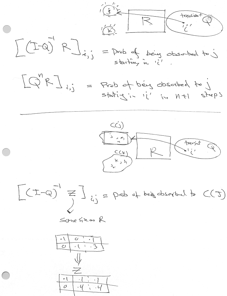
$f = [(I − Q )−1 R] ij i,j$

$i ∈ T j ∈ T$

We know eventually $pij = 0$ for $i,j ∈ Q$ , but can we talk about $fij$ here?

3.3 How to find $E (Vij)$ the expected number of visits to j before absorbing?

The above gives the average number of visits to state $j$ (also transient) before chain is absorbed for first time.

question: Note that if chain is regular, then all states communicates with each others and then $i ∈ R, j ∈ R$ and so $E (Vij)$ can be found from the stationary distribution $π ∞$ , right?

3.4 How to find average number of steps $E (Tij)$ between state $i$ and state $j$ ?

3.5 How to find number of visits to a transient state?

where $fii$ is the probability of visiting state $i$ if chain starts in state $i$

4 Some useful formulas

4.1 Law of total probability

4.2 Conditional (Bayes) formula

4.3 Inverse of a 2 by 2 matrix

4.4 $ω = 1- j μj$

The above says that for a regular finite MC, where a stationary probability exist (and is unique), then it is inverse of the mean number of steps between visits $μj$ to state $j$ in steady state.

4.5 $ω = ωP$

The above says that for a regular M.C. there exist a stationary probability distribution $ω$

4.6 Poisson random variable

Where $λ$ is the average number of events that occur over the same period that we are asking for the probability of this number of events to occur. Hence remember to adjust $λ$ accordingly if we are given $λ$ as rate (i.e. per unit time).

4.7 Poisson random Process

Where $λ$ is the average number of events that occur in one unit time. So $N (t)$ is random variable which is the number of events that occur during interval of length $t$

The probability that ONE event occure in the next $h$ interval, when the interval is very small, is $λh + o(h )$

This can be seen by setting $n = 1$ in the definition and using series expansion for $− (λh) e$ and then letting $h → 0$

Expected value of Poisson random variable: $E (N ) = λ$ . For a process, $E (N (t)) = λt$ where $λ$ is the rate.

4.8 Exponential random variable

$T$ is random variable which is the time between events where the number of events occur as Poisson distribution,

$∫t −λs [ −λs]t [ −λt ] − λt P (T < t) = λe ds = − e 0 = − e − 1 = 1 − e 0$

pdf=derivative of CDF

Probability that the waiting time for $n$ events to occur $≤ t$ is a GAMMA distribution. $gn (t) = (nλ−1)! (λt)n−1e− λt$

5 Diagram to help understanding

5.1 Continouse time Markov chain

$vi$ is the parameter (rate) for the exponential distributed random variable which represents the time in that state. Hence The probability that system remains in state $i$ for time larger than $t$ is given by

$∘)$ Jump probability $Qij = qij vi$ for $i ⁄= j$ . This is the probability of going from state $i$ to state $j$ (once the process leaves state $i$ )

$P ′(t) = P (t) Q$ , let $z (t) = z (0)P (t)$ , hence $z′(t) = z (0)P ′(t),$ hence $z′(t) = z (0)P (t)Q$ therefore

This equation can also be obtaind more easily I think from $πQ = 0$ Where $Q$ is the matrix made up from the $q ′s$ and the $v ′s$ on the diagonal. Just write then down, and at the end add $π0 + π1 + ⋅⋅⋅ = 1$ to find $π0$


$regular : i ∈ R, j ∈ R$	$∑ E (Tij) = 1 + pikE (Tkj) k⁄=j if i = j then E (Tij) = w1jj where w is the stationary probability vector$

$i ∈ T, j ∈ T$	does not make sense to ask this here?