3.1 Solution
3.1.1 Introduction
current database for the bridge, in the format of SDB SAP2000 1.5 version is SBD
file
Results of each step are given in separate section. Each section has two parts, the first shows the
results and the second describes the methods and analysis performed to obtain the
results.
3.1.2 step one. Displacements at joints S15L, S07L and 21
3.1.2.1 Results
| | | | | | |
| Joint |
U1 |
U2 |
U3 |
R1 |
R2 |
R3 |
| |
ft | ft | ft | rad | rad | rad |
| | | | | | |
| S07L | 0.000179 | -0.003174 | 0.021538 | -0.000119 | 0.000098 | 4.253E-06 |
| S15L |
0.000035 |
-0.003104 |
-0.032437 |
-0.000216 |
-0.001357 |
0.000029 |
| | | | | | |
| | | | | | |
| Joint |
U1 |
U2 |
U3 |
R1 |
R2 |
R3 |
| |
ft | ft | ft | rad | rad | rad |
| | | | | | |
| 21 | 0.007568 | -0.002749 | -0.024066 | -0.000011 | 0.001533 | -0.000120 |
| | | | | | |
Table 3.1: Displacements at joint 21
3.1.2.2 Method used
Problem description is
Find the deflections of the arch portion of the bridge at node or joint S15L and S07L when
a 10k downward point load is applied at joint S15L. Also find the displacements of joint 21
on the ramp when a 10k downward load is applied at that joint.
There are the steps performed
- The original bridge database was not complete. The missing joints were first added.
After opening the database, the XZ view was selected. This is needed as it was found
it is not possible to add a point in the default 3D view.
- Clicked on the Draw Special joint icon located on the left edge of the window.
This is the small blue square in version 15 of SAP2000.
- Clicked on an empty area on the screen to add a point.
- Right clicked on the added point again to bring up a pop-up menu dialogue that was
used for data entry of given coordinates.
- Filled the coordinates and the labels as given in the PDF file.
- Made sure that the menu item in the JOINT COORDINATES called
SPECIAL Jt (User Def) is labeled YES. If this is labeled NO then this procedure did
not work and the point was not added.
- Clicked UPDATE DISPLAY then clicked OK.
- Verified that the points were added by selecting DISPLAY->SHOW TABLES then using
the pop-up menu and searched Joint Coordinates
-
Figure 3.1 shows part of the joints coordinates table after completing the above steps.
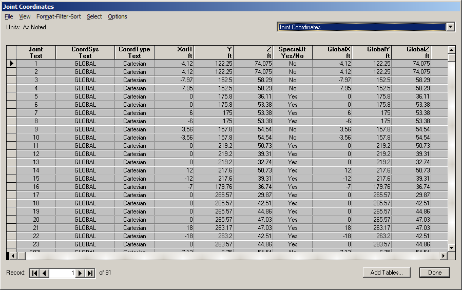 Figure 3.1: Adding missing joints to bridge database
Partial listing of joints is shown below
SAP2000 v15.0.1    5/2/13 22:18:29
Table:  Joint Coordinates
       Joint          CoordSys   CoordType        XorR           Y           Z   SpecialJt     GlobalX     GlobalY     GlobalZ
                                                    ft          ft          ft                      ft          ft          ft

           1            GLOBAL   Cartesian     -4.1200    122.2500     74.0750          No     -4.1200    122.2500     74.0750
           2            GLOBAL   Cartesian      4.1200    122.2500     74.0750          No      4.1200    122.2500     74.0750
           3            GLOBAL   Cartesian     -7.9700    152.5000     58.2900          No     -7.9700    152.5000     58.2900
           4            GLOBAL   Cartesian      7.9500    152.5000     58.2900          No      7.9500    152.5000     58.2900
           5            GLOBAL   Cartesian      0.0000    175.8000     36.1100         Yes      0.0000    175.8000     36.1100
           6            GLOBAL   Cartesian      0.0000    175.8000     53.3800         Yes      0.0000    175.8000     53.3800
           7            GLOBAL   Cartesian      6.0000    175.0000     53.3800         Yes      6.0000    175.0000     53.3800
           8            GLOBAL   Cartesian     -6.0000    175.0000     53.3800         Yes     -6.0000    175.0000     53.3800
           9            GLOBAL   Cartesian      3.5600    157.8000     54.5400          No      3.5600    157.8000     54.5400
          10            GLOBAL   Cartesian     -3.5600    157.8000     54.5400          No     -3.5600    157.8000     54.5400
          11            GLOBAL   Cartesian      0.0000    219.2000     50.7300         Yes      0.0000    219.2000     50.7300
          12            GLOBAL   Cartesian      0.0000    219.2000     39.3100         Yes      0.0000    219.2000     39.3100
          13            GLOBAL   Cartesian      0.0000    219.2000     32.7400         Yes      0.0000    219.2000     32.7400
          14            GLOBAL   Cartesian     12.0000    217.6000     50.7300         Yes     12.0000    217.6000     50.7300
          15            GLOBAL   Cartesian    -12.0000    217.6000     39.3100         Yes    -12.0000    217.6000     39.3100
          16            GLOBAL   Cartesian     -7.0000    179.7600     36.7400         Yes     -7.0000    179.7600     36.7400
          17            GLOBAL   Cartesian      0.0000    265.5700     29.8700         Yes      0.0000    265.5700     29.8700
          18            GLOBAL   Cartesian      0.0000    265.5700     42.5100         Yes      0.0000    265.5700     42.5100
          19            GLOBAL   Cartesian      0.0000    265.5700     44.8600         Yes      0.0000    265.5700     44.8600
          20            GLOBAL   Cartesian      0.0000    265.5700     47.0300         Yes      0.0000    265.5700     47.0300
          21            GLOBAL   Cartesian     18.0000    263.1700     47.0300         Yes     18.0000    263.1700     47.0300
          22            GLOBAL   Cartesian    -18.0000    263.2000     42.5100         Yes    -18.0000    263.2000     42.5100
          23            GLOBAL   Cartesian      0.0000    283.5700     44.8600         Yes      0.0000    283.5700     44.8600
-
Connected the joints added above to the bridge in order to establish the ramp. Figure 3.2
is screen shot showing the ramp connected to bridge. RBEAM elements are used.
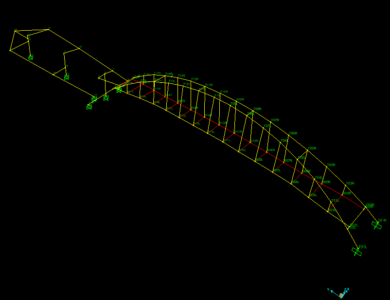 Figure 3.2: connected ramp to bridge using RBEAMS
- Before adding the 10 kips downwards load, a load pattern is defined. Selected
DEFINE->LOAD PATTERNS and added new load pattern called S15L of type DEAD with self
weight multiplier 0.
-
10 kips downwards load at joint S15L was added. This was done by clicking on the joint
and right clicking again. Using the pop up menu that appeared the value minus 10 was
entered. Minus sign was used since load is downwards. The load pattern selected was S15L.
Figure 3.3 shows the result.
 Figure 3.3: adding vertical load pattern for step one use
-
Clicked on RUN ANALYSIS. In the set load case to run case S15L was the only one
selected. All other load cases, including DEAD was not selected. This was done to obtain
result due to vertical load only. Model was locked now. After run was completed, clicked on
DISPLAY->SHOW TABLES->JOINT DISPACEMENTS and located nodes S15L and
S07L to find the node displacements. Figure 3.4 shows the result of this step
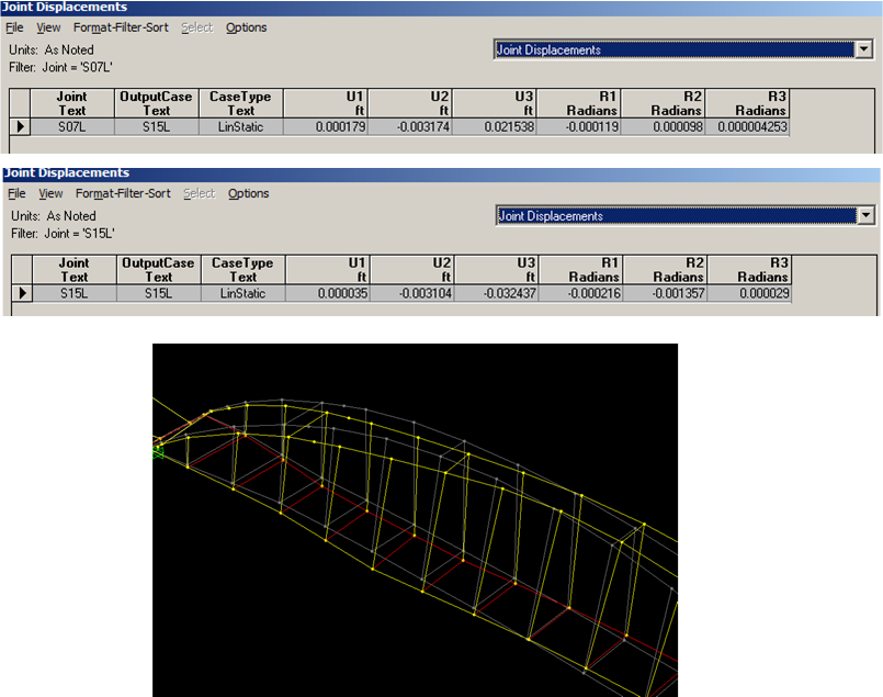 Figure 3.4: adding vertical load to joint S15L
In addition a listing from the table is shown below
SAP2000 v15.0.1    5/3/13 1:35:52
Table:  Joint Displacements
 Joint OutputCase  CaseType      U1         U2         U3         R1        R2        R3
                                 ft         ft         ft     Radians     Radians   Radians

 S07L    S15L    LinStatic    0.000179  -0.003174   0.021538  -0.000119   0.000098  4.253E-06
 S15L    S15L    LinStatic    0.000035  -0.003104  -0.032437  -0.000216  -0.001357  0.000029
- Before adding the 10 kips downwards load to node 21, a load pattern is defined for use.
Selected DEFINE->LOAD PATTERNS and added new load pattern called node21 of type DEAD
with self weight multiplier 0.
-
10 kips downwards load at joint 21 was now added. This was done by clicking on the joint
and right clicking aging. Using the pop-up menu that appeared the value minus 20 was
entered. Minus sign was used since load is downwards. The load pattern selected was
node20. Figure 3.5 shows this step.
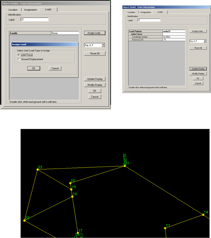 Figure 3.5: adding vertical load pattern for step one use
-
Clicked on RUN ANALYSIS. In the setload case to run case node21 was the only
one selected. All other load cases, including DEAD was not selected. This was
done to obtain result due to vertical load only. Model was locked now. After run
was completed, clicked on DISPLAY->SHOW TABLES->JOINT DISPACEMENTS and
located nodes 21 to find the node displacements. Figure 3.6 shows the result.
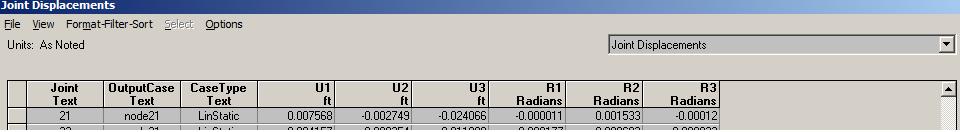 Figure 3.6: adding vertical load to joint 21
Listing from the table is shown below
SAP2000 v15.0.1    5/3/13 2:33:04
Table:  Joint Displacements
 Joint  OutputCase  CaseType      U1         U2         U3        R1        R2        R3
                                  ft         ft         ft     Radians    Radians   Radians

  21      node21    LinStatic   0.007568  -0.002749  -0.024066  -0.000011 0.001533  -0.000120
3.1.3 Step two, period and damping calculations
3.1.3.1 Results
The result is shown in table 3.2
| | |
| Natural period \(T\) (sec) | Natural frequency \(f_n\) (hz) | critical damping ratio \(\zeta \) |
| | |
| 0.5 | 2.0 | 0.0014% |
| | |
Table 3.2: Period and damping
3.1.3.2 Method used
This is the problem description
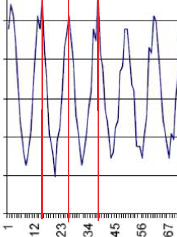
Two people jogging across the bridge created the vertical acceleration records shown below.
Each set of pulses is when the joggers were running, in between they stopped. Once they
stopped it is as if the bridge had an initial displacement and velocity and then decayed in
free vibration. Using the enlarged portion of the record estimate - the natural period of the
structure and the
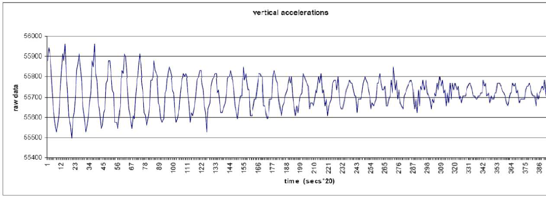 Figure 3.7: vertical acceleration time records
The above profile can be used as free the vibration profile. The method of logarithmic decrement
was used to obtain the natural period and \(\zeta \) (damping critical coefficient). Figure 3.8 shows a
closer zoom view of the above plot in order to estimate the period. It shows the natural period to
be around 10 division.
 Figure 3.8: zoomed view on the vertical acceleration time records
The units used are sec*20, therefore natural period is \(T=\frac {10}{20}=0.5\) sec. Hence natural frequency is \(f=2\)
hz.
To obtain the damping \(\zeta \), a number of methods can be used. The more accurate methods uses
more peaks. Using \(N=35\) as number of peaks and using method of series expansion \(\zeta \) can be found. From
the above plot the value of first peak is 55940 and value of peak number 35 was found to be
55770. Hence \begin {align*} \frac {y_0}{y_0+N} & = 1 + 2\pi N \zeta \\ \zeta & = \frac {1}{35(2\pi )} \frac {55940-55770}{55770}\\ & = 1.3861 \times 10^{-5}\\ & = 0.0014 \% \end {align*}
3.1.4 Step three. Modal analysis
3.1.4.1 Results
The following are the modal analysis results. Mode 3 has period 0.426531 seconds and natural
frequency 2.3445 hz.
SAP2000 v15.0.1    5/3/13 3:29:56
Table:  Modal Periods And Frequencies

 OutputCase    StepType  StepNum     Period   Frequency    CircFreq  Eigenvalue
                                      Sec      Cyc/sec      rad/sec   rad2/sec2

  Modal        Mode    1.000000    0.486993  2.0534E+00  1.2902E+01  1.6646E+02
  Modal        Mode    2.000000    0.435780  2.2947E+00  1.4418E+01  2.0789E+02
  Modal        Mode    3.000000    0.426531  2.3445E+00  1.4731E+01  2.1700E+02
  Modal        Mode    4.000000    0.352227  2.8391E+00  1.7838E+01  3.1821E+02
  Modal        Mode    5.000000    0.321345  3.1119E+00  1.9553E+01  3.8231E+02
  Modal        Mode    6.000000    0.268232  3.7281E+00  2.3424E+01  5.4871E+02
  Modal        Mode    7.000000    0.258425  3.8696E+00  2.4313E+01  5.9114E+02
  Modal        Mode    8.000000    0.249385  4.0099E+00  2.5195E+01  6.3477E+02
In this description, reference is made to different view angles. Figure 3.48 shows the axis
orientation used by SAP2000.
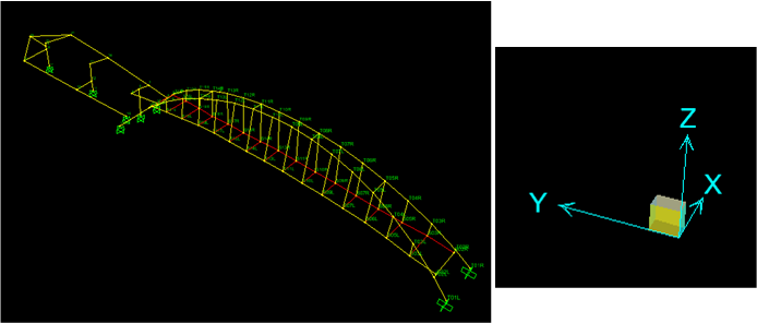 Figure 3.9: 3D axis orientation used
The maximum stress at the base of the column (label 11) in the ramp was also found for each
mode. This was done using SAP2000 v15.1 which has this added feature. The following diagrams
give stress S11 for each mode.
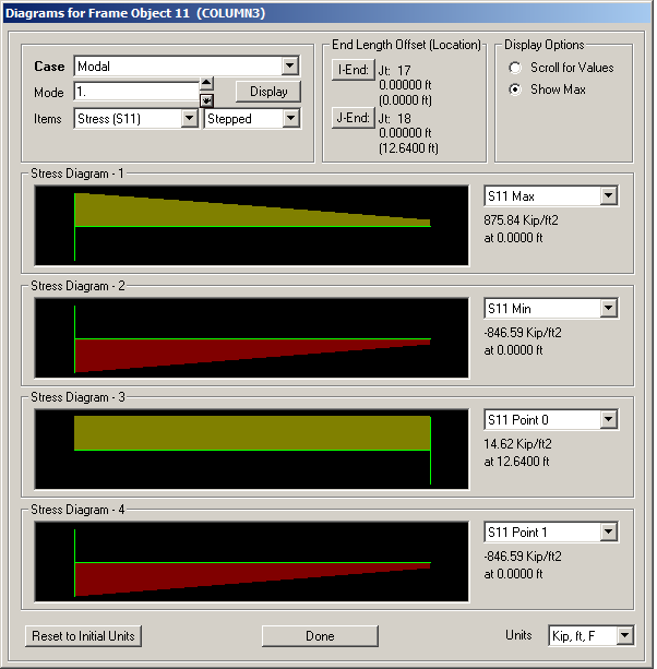 Figure 3.10: Stress at base of column, mode 1
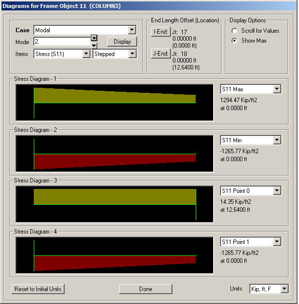 Figure 3.11: Stress at base of column, mode 2
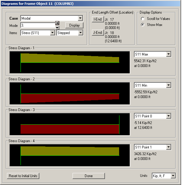 Figure 3.12: Stress at base of column, mode 3
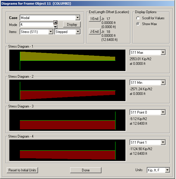 Figure 3.13: Stress at base of column, mode 4
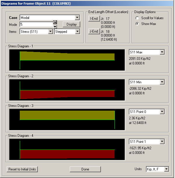 Figure 3.14: Stress at base of column, mode 5
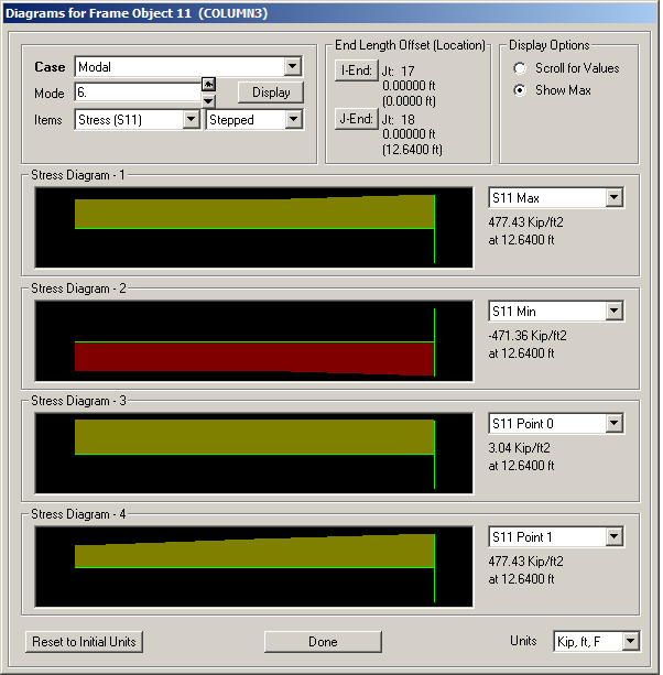 Figure 3.15: Stress at base of column, mode 6
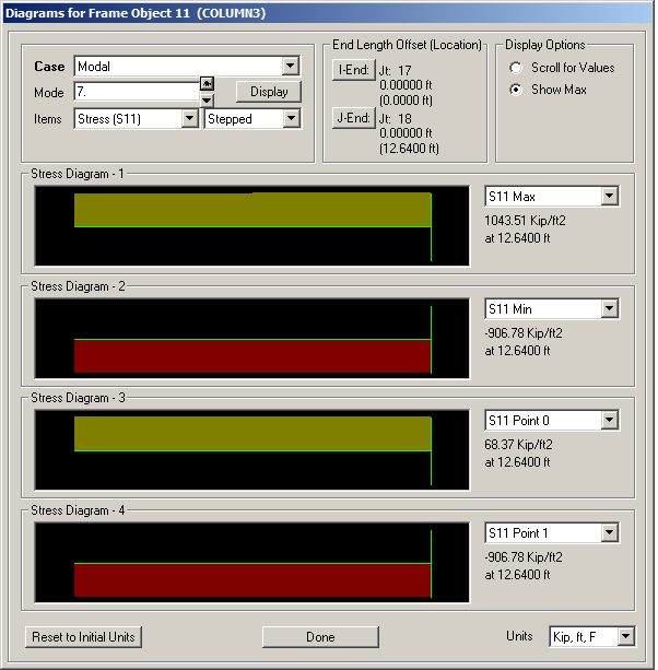 Figure 3.16: Stress at base of column, mode 7
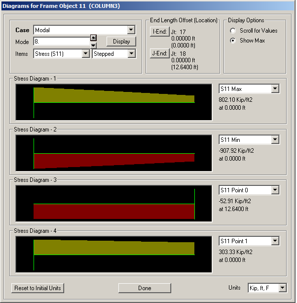 Figure 3.17: Stress at base of column, mode 8
3.1.5 Step four. Solving for response under simulated marching band
3.1.5.1 Results
The nodes to find the displacements for are marked and given in figure ?? .
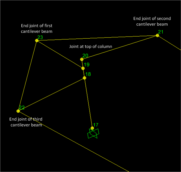 Figure 3.18: node locations for cantilever beams
The result is shown below. The labels for local axes for joints are shown below, and are the same
as the global axes. This is from SAP2000 help section
  By default, the joint local 1-2-3 coordinate system is identical to
  the global X-Y-Z coordinate system
Therefore, U1 is in the X direction, and U2 in the Y direction, and U3 is the vertical
displacement.
SAP2000 v15.0.1    5/4/13 1:02:04
Table:  Joint Displacements
 Joint  OutputCase  StepType    U1          U2          U3          R1          R2          R3
                                ft          ft          ft        Radians     Radians     Radians
  20      COMO       Max     0.146711    0.019285   -0.000479    0.001667    0.015544    0.000542
  20      COMO       Min    -0.141382   -0.017992   -0.000676   -0.001788   -0.013209   -0.000675

  21      COMO       Max     0.144476    0.034315    0.262294    0.002986    0.022603    0.001017
  21      COMO       Min    -0.139764   -0.037636   -0.375865    0.000383   -0.015478   -0.001261

  22      COMO       Max     0.082805    0.009682    0.236030    0.003108    0.014103   -0.000012
  22      COMO       Min    -0.083333   -0.005028   -0.305074   -0.000501   -0.018799   -0.000326

  23      COMO       Max     0.123308    0.015499    0.013802    0.001111    0.015690    0.000583
  23      COMO       Min    -0.123593   -0.014890   -0.049072   -0.002825   -0.014603   -0.000494
Figure 3.19 shows screen shot of the deformed part of the ramp with the above joints marked on
the diagram showing the relative displacement for better illustration.
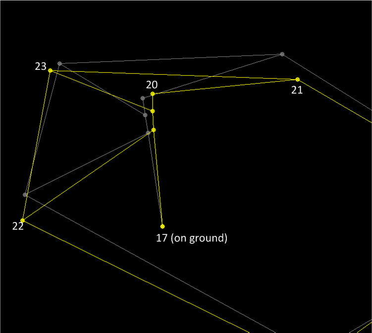 Figure 3.19: relative displacements of joints on ramp
The following text file contains the result for all nodes. step_4_beam_result.txt
In addition, below are plots of nodal displacements of node 20, on top of column labeled 11 on
the ramp (this is the column being analyzed for stress). This plot shows that it took about 20
seconds for dynamic loading to settle down.
This means after 20 second of the marching band moving into the ramp, the ramp vibration
reached steady state, therefore, the ramp is now vibrating at the same forcing frequency and
transient response of the ramp has completed.
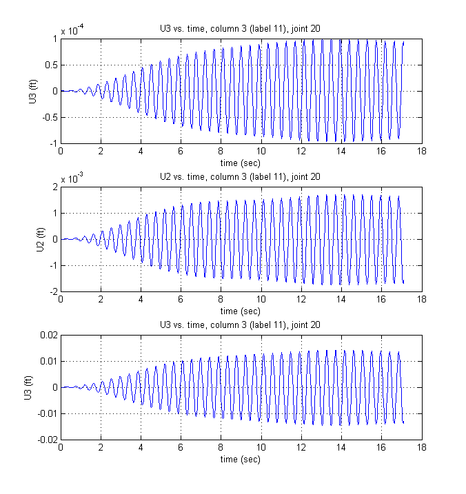 Figure 3.20: Displacement of node 20 on ramp column 3 during dynamic response
This is a plot the total axial load \(P\) on the column for the first 20 seconds.
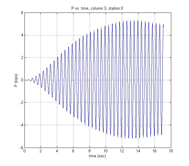 Figure 3.21: Axial load \(P\) variation in column during during dynamic excitation
This is movie of the first 20 seconds of the bridge vibration during marching band motion.
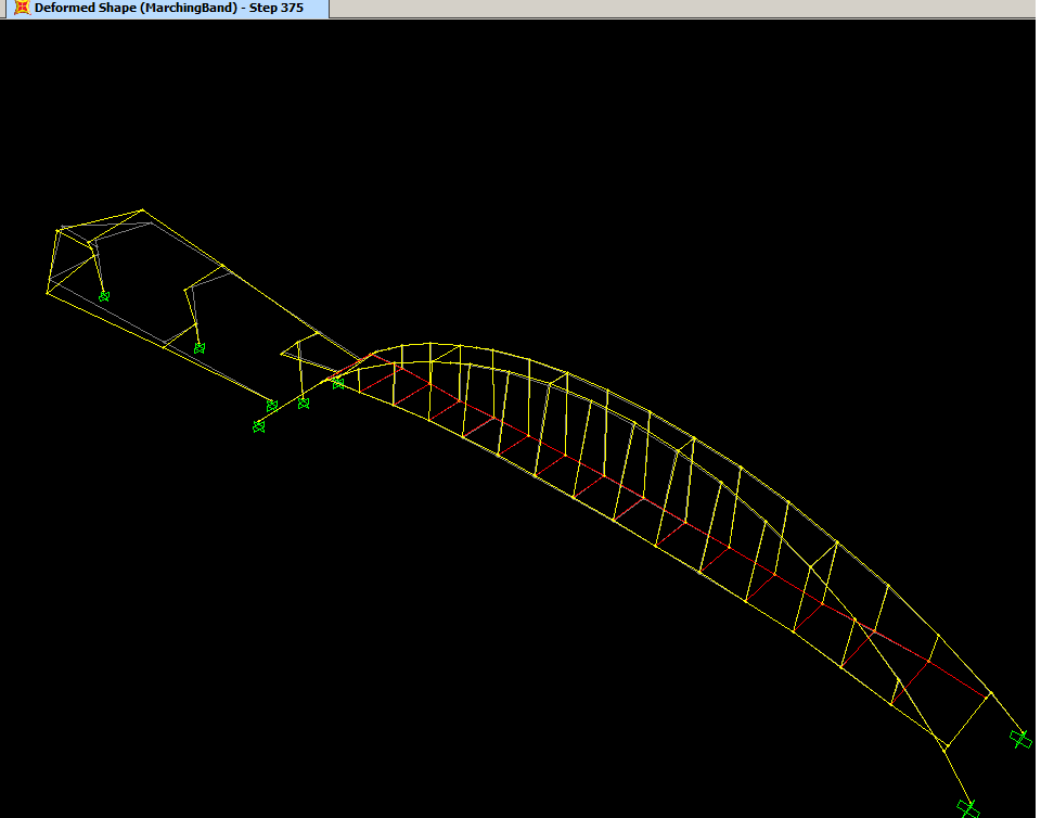 Figure 3.22: movie of first 20 seconds during marching band motion
Node displacement for joint 20 under marching band (time history) is given below. The output is
in this file node_20_final_displacement.txt
This is partial listing of the table from SAP2000.
SAP2000 v15.0.1    5/3/13 5:24:47
Table:  Joint Displacements

 Joint  OutputCase   CaseType    StepType  StepNum      U1          U2          U3          R1          R2          R3
                                                        ft          ft          ft        Radians     Radians     Radians

   20 MarchingBand  LinModHist     Time    0.000000   0.000000    0.000000    0.000000    0.000000    0.000000    0.000000
   20 MarchingBand  LinModHist     Time    0.021400  -3.745E-07   6.625E-08   2.712E-10  -7.568E-09  -3.795E-08   2.215E-09
   20 MarchingBand  LinModHist     Time    0.042800  -2.849E-06   5.016E-07   2.063E-09  -5.715E-08  -2.887E-07   1.677E-08
   20 MarchingBand  LinModHist     Time    0.064200  -8.717E-06   1.522E-06   6.310E-09  -1.726E-07  -8.828E-07   5.090E-08
   20 MarchingBand  LinModHist     Time    0.085600   -0.000018   3.074E-06   1.289E-08  -3.463E-07  -1.804E-06   1.028E-07
3.1.5.2 Method
Description of the problem is given below
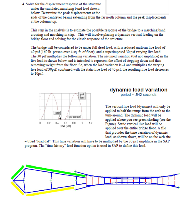 Figure 3.23: Description of step 4, solving for response under dynamic marching band
The following are the steps performed
-
Load patterns are first defined. In SAP2000, a load case uses a load pattern. Hence
a load pattern must first be be defined. Load pattern tells SAP where the loads are
while a load cases tells SAP how to apply a specific load pattern, for example, either
statically or dynamically and also tells SAP how to perform the analysis, for example,
either using modal or direct integration.
Figure 3.24 shows the relation between load patterns and load cases as used in
SAP2000.
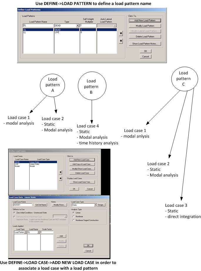 Figure 3.24: Relation between load pattern and load case
The first load pattern is live load. This is the load of people on the bridge and is present all
the time. The bridge is 10 ft wide, and the problem says to use 40 lb per square feet, or 400
lb per linear feet.
Selected DEFINE->LOAD PATTERNS and wrote LL in the Load Pattern Name
window. selected LIVE as type, and set self weight multiplier to 0 then clicked
Add New Load Pattern. Figure 3.25 shows this step.
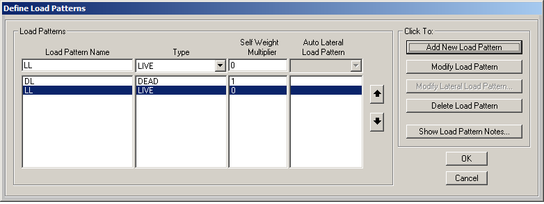 Figure 3.25: Defining live load pattern LL
- Defined a new load pattern similar to the above called DYNALOAD of type LIVE and also a
self weight of zero.
-
Selected the floor of the bridge using SELECT->PROPERTIES->AREA SECTIONS->FLOOR.
Added load LL using ASSIGN->AREA LOADS->UNIFORM(SHELL) and selected LL for load
pattern. Used 0.04 for the load amount. This is 40 psf. (or 400 lb per linear ft, since the
bridge is 10 ft wide). Figure 3.26 shows this step.
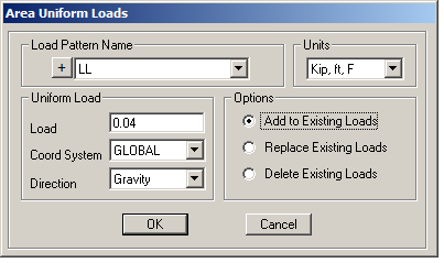 Figure 3.26: Adding live load to bridge floors
-
added 400 lb per linear ft also to on the ramp. SELECT->PROPERTIES->FRAME SECTIONS->RBEAM
and as the ramp is selected clicked ASSIGN->FRAME LOAD->DISTRIBUTED LOAD and entered
400 (lb per linear ft). Load pattern LL was used. Figure 3.27 shows this step.
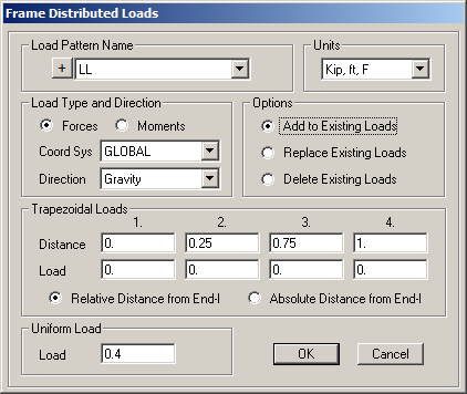 Figure 3.27: Adding LL load to ramp RBEAMs
-
Added 10 kips per linear ft as distributed load on the first 4 RBEAMS on the right side of
the ramp. Selected DYNALOAD as the load definition. Figure 3.28 shows this step.
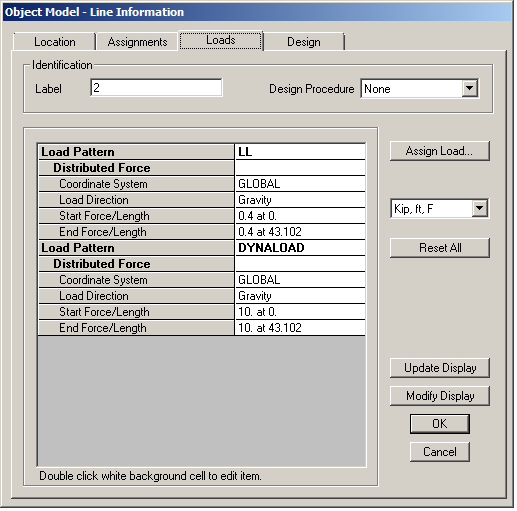 Figure 3.28: Adding 10 kips load on right side of RAMP
-
Using the menu, selected DEFINE->FUNCTIONS->TIME HISTORY then selected From file
and clicked on Add New Function... and gave it name and used the browser to locate the
text file that contains the time history. The time history file was downloaded from the class
web site.
Set VALUES AT EQUAL INTERVALS to 0.0214. Figure 3.29 shows this step.
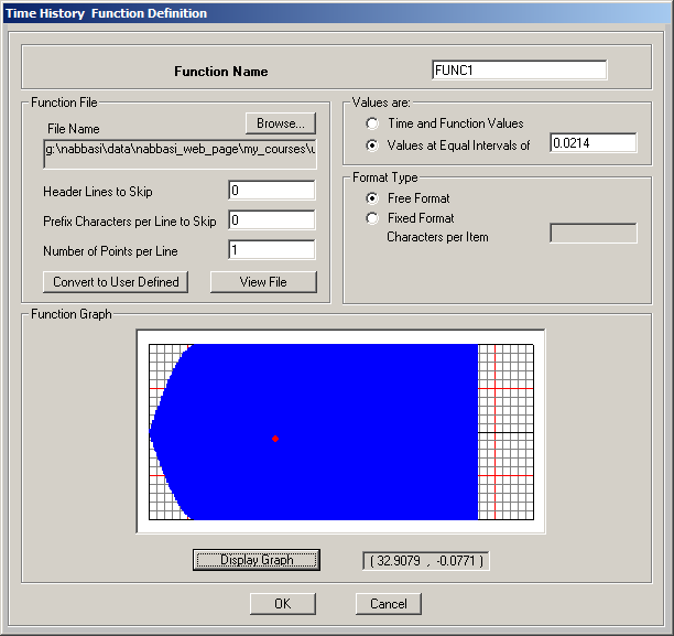 Figure 3.29: Adding time history function
-
Defined MODAL load case. Selected EIGN VECTOR and not RITZ Figure 3.30 shows this step.
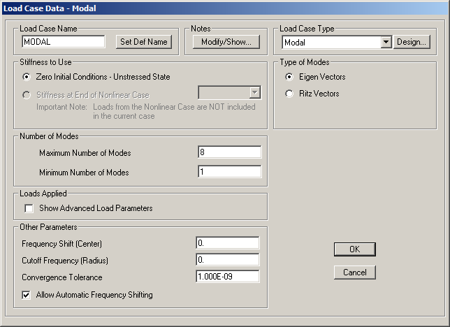 Figure 3.30: Adding MODAL load case
-
Defined load case MarchingBand to use for time history loading to simulate the marching
band on the ramp. Selected DYNALOAD as load pattern. Made sure to change the scale to
0.03. Figure 3.31 shows this step.
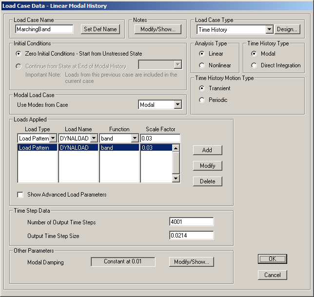 Figure 3.31: defining marching band dynamic load case
-
Defined a COMBINATION load case called COMO as shown in Figure 3.32
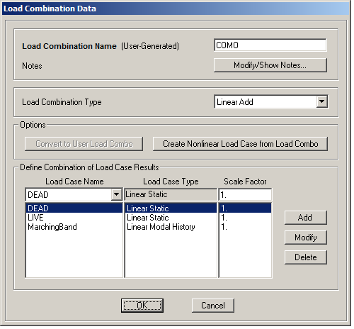 Figure 3.32: defining combination load case
-
Modified mass and weight property of RBEAM by changing property modifier
mass to 2.1762 and property modifier weight to 2.1748 as shown in Figure 3.33
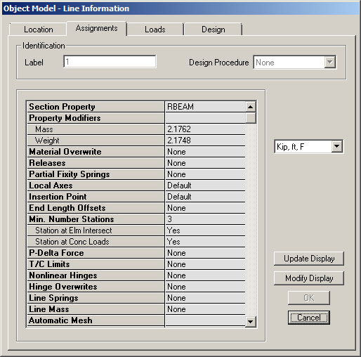 Figure 3.33: modified section property RBEAM
-
PEAK DISPLACEMENT at end of cantilever beams extending from far north column are
found. These are the sections called CANT3. The first beam is from node 20 to
21, the second beam from node 23 to 19, and the third beam from node 22 to
18.
Clicked on run and selected all cases to run. When run was completed, clicked on
Display->Tables and clicked on Select load cases... and selected COMO. Then selected
ANALYSIS RESULTS followed by Joint Output->Displacements->Table.
Searched the table of joint Displacements for the 3 beams given above.
- Wrote a Matlab script to plot the time history displacement for node 20 under marching
band motion is in this file sap_post_processes.m
3.1.6 Step five. Stress results
3.1.6.1 Results
In this step, peak stress calculations at the bottom of came column under the peak marching
band are made. A Matlab script was written to do the computation based on result obtained
from SAP tables.
Maximum tensile and compressive stress due to marching band load only was first found. Then
the stress due to dead and live load was added as a separate step. The final result is show on
table 3.3
| | |
| load case |
max compressive stress (kip/sq inch) |
max tensile stress (kip/sq inch) |
| | |
| | |
| marching band (4001 steps) |
-44.125 |
45.24 |
| | |
| dead load | -1.3812 | |
| | |
| live load |
-0.519 |
|
| | |
| combined |
-46.02 |
45.24 |
| | |
| | |
Table 3.3: Stress calculation result for step 5
Figure 3.34 shows variation of stress during the 85 seconds of the time history of the marching
band.
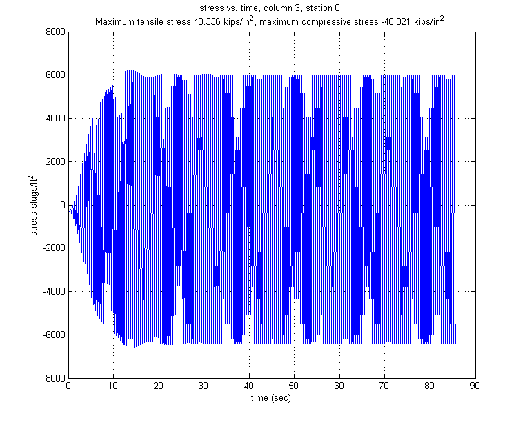 Figure 3.34: Plot of stress vs. time during dynamic loading
3.1.6.2 additional results
Additional analysis was done using SAP2000 V15.1 which allows one to visually examine stress
diagrams. By selecting this Show stress and selecting this column and point 17 (which is station
0) which is the base of the column, the following diagrams are obtained for different measures at
this location. However, these results are obtained before changing the section module of the
column to the one we are asked to used in this project. Hence the results shown are not the same
found above due to this. These are left here for reference and illustration of this SAP2000 feature.
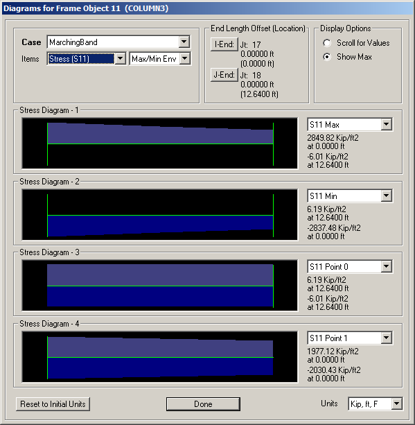 Figure 3.35: max/min of S11 stress at base of column, Marching band case
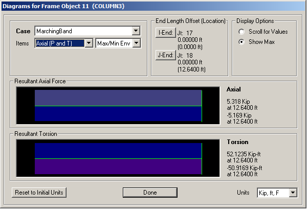 Figure 3.36: Max/min of axial load at base of column, Marching band case
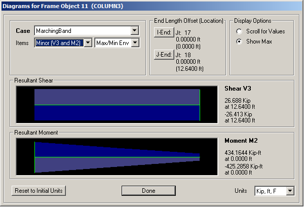 Figure 3.37: Max/min \(M_{22}\) at base of column, Marching band case
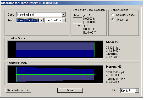 Figure 3.38: Max/min \(M_{33}\) at base of column, Marching band case
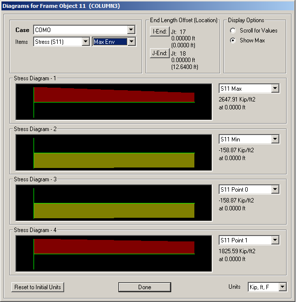 Figure 3.39: Stress S11 at base of column, Combination test case
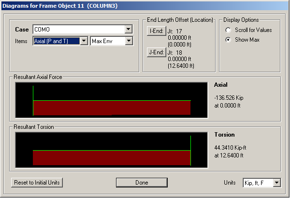 Figure 3.40: Axial load at base of column, Combination test case
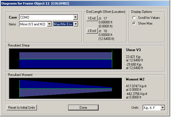 Figure 3.41: Max/min \(M_{22}\) at base of column, Combination test case
 Figure 3.42: Max/min \(M_{33}\) at base of column, Combination test case
3.1.6.3 Method
- Selected run with all load cases.
- Selected Display-Show Tables-Analysis Results-Element Output-Frame Output-Element Forces
Modify/Show Options.. was used to make sure the envelope option is not selected
and that the step-by-step option is selected under the Modal History Results.
Also made sure that the load case MarchingBand and COMO are the only ones selected.
- Waited for table to build. This took about 30 minutes. Then used the table filter to
select column 11 and station 0 (this is the bottom of the column).
- Saved the table to a text file to process using Matlab. Here is the text file that
contains the results. final_station_zero_forces.txt
-
Now obtained the stress due to dead load and dynamic load. This was done by
running the analysis again and now selecting LIVE and DEAD load cases and using
the envelope. The result is in this file final_load_result_DEAD_and_LIVE.txt
SAP2000 v15.0.1    5/8/13 2:08:08
Table:  Element Forces - Frames

 Frame     Station  OutputCase    CaseType           P          V2          V3           T          M2          M3      S11Max    PtS11Max    x2S11Max    x3S11Max      S11Min    PtS11Min    x2S11Min    x3S11Min   FrameElem ElemStation
                ft                                 Kip         Kip         Kip      Kip-ft      Kip-ft      Kip-ft     Kip/ft2                      ft          ft     Kip/ft2                      ft          ft                      ft

    11      0.0000        DEAD   LinStatic    -101.634       0.257      -3.227     -6.3522    -19.2532     26.2485      -81.17           2    -0.50000     0.50000     -155.36           3     0.50000    -0.50000        11-1      0.0000
    11      0.0000        LIVE   LinStatic     -40.210       0.082      -0.040     -1.4303      2.1635     14.0489      -34.51           1    -0.50000    -0.50000      -59.07           4     0.50000     0.50000        11-1      0.0000
- Ran the Matlab script and obtained the maximum stress. The area for the column cross
section is 0.8594 square ft. The matlab script is in this file stress_calc.m
- Calculation used for stress is based on the following formula \( \sigma = \frac {P}{A} \pm \frac {M_{22}}{0.536} \pm \frac {M_{33}}{0.586} \) Where \(A\) is the section area of
the beam and \(M_{22}\) and \(M_{33}\) are the internal bending moments at the base of the column obtained
from SAP2000 finite elements results. Final stress was converted from kip per sq ft to kip
per sq inch by dividing by 144.
3.1.7 Appendix
3.1.7.1 SAP2000 definitions used in this report
These below are obtained from SAP2000 help sections.
Local axis signs
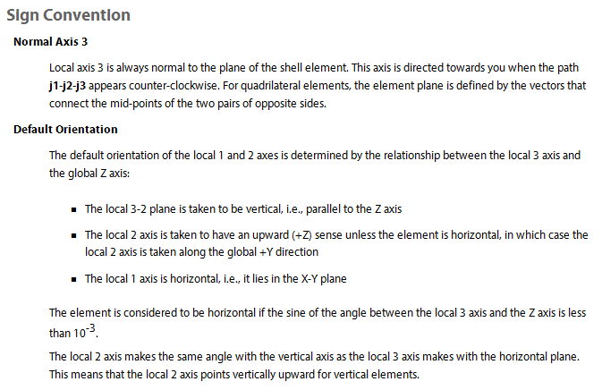 Figure 3.43: SAP2000 local axis signs
Frame element internal forces output convention
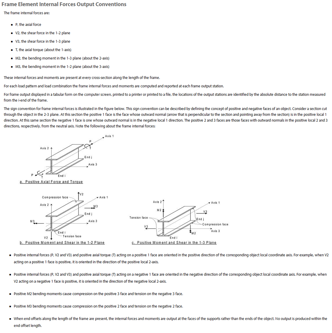 Figure 3.44: SAP2000 Frame element internal forces output convention
SAP2000 S11 description (stress calculations)
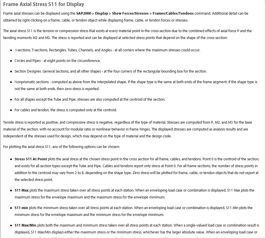 Figure 3.45: SAP2000 S11 description
SAP2000 shell element internal forces/stresses output convention
 Figure 3.46: SAP2000 shell element internal forces/stresses output convention
3.1.7.2 references
- Lecture notes given by professor Michael G. Oliva, college of engineering, dept. of
civil engineering. CEE 744 structural dynamics, spring 2013.
- SAP2000 The modeling and analysis of human-induced vibrations due to footfalls or
another type of impact.
- Structural vibrations which result from human footfalls may be modeled in ETABS
using modal time-history analysis
- Description of joints in SAP2000 https://wiki.csiberkeley.com/display/kb/Joint
These below are documents that describe the project itself and SAP 2000 guide and the original
SAP model we obtained to start from.
- Problem statment for Elizabeth Ashman Bridge CEE744Ashman2013.pdf
- Original SAP 2000 data file ashdynstat_original.sdb
- SAP 2000 GUIDE SAPGuide.pdf