• up
• This page in PDF

Contents

Matlab files used

1.

problems as1.pdf

1 Problem 1.1 page 9

Answer

1.1 part a

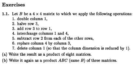
Operations that acts on columns of \(B\) are implemented using a matrix which is post multiplied by \(B\), while operations that acts on rows of \(B\) are implemented by a matrix which is pre multiplied by \(B\).

1.

To double the first column of a \(4\times 4\) matrix \(B\), it is post multiplied by\[ C_{1}=\begin{pmatrix} 2 & 0 & 0 & 0\\ 0 & 1 & 0 & 0\\ 0 & 0 & 1 & 0\\ 0 & 0 & 0 & 1 \end{pmatrix} \] Hence \(B\times C_{1}\)

2.

To halve row 3 of a \(4\times 4\) matrix \(B\), it is pre multiplied by\[ R_{1}=\begin{pmatrix} 1 & 0 & 0 & 0\\ 0 & 1 & 0 & 0\\ 0 & 0 & \frac{1}{2} & 0\\ 0 & 0 & 0 & 1 \end{pmatrix} \] Hence \(R_{1}\times B\)

To add row 3 to row 1 of \(4\times 4\) matrix \(B\), it is pre multiplied by a matrix with diagonal all ones, and with \(1\) in the third column of the first row\[ R_{2}=\begin{pmatrix} 1 & 0 & 1 & 0\\ 0 & 1 & 0 & 0\\ 0 & 0 & 1 & 0\\ 0 & 0 & 0 & 1 \end{pmatrix} \] Hence \(R_{2}\times B\)

To interchange columns 1 and 4 of \(4\times 4\) matrix \(B\), it is post multiplied by a matrix with diagonal that has 1 for those columns that should remain as is, and with 1 in \(C(4,1)\) and 1 in \(C(1,4)\) as follows\[ C_{2}=\begin{pmatrix} 0 & 0 & 0 & 1\\ 0 & 1 & 0 & 0\\ 0 & 0 & 1 & 0\\ 1 & 0 & 0 & 0 \end{pmatrix} \] Hence \(B\times C_{2}\)

To subtract row 2 from each of the other 3 rows of \(4\times 4\) matrix \(B\), it is pre multiplied by\[ R_{3}=\begin{pmatrix} 1 & -1 & 0 & 0\\ 0 & 1 & 0 & 0\\ 0 & -1 & 1 & 0\\ 0 & -1 & 0 & 1 \end{pmatrix} \] Hence \(R_{3}\times B\)

To replace column 4 by column 3 \(4\times 4\) matrix \(B\), it is post multiplied by\[ C_{3}=\begin{pmatrix} 1 & 0 & 0 & 0\\ 0 & 1 & 0 & 0\\ 0 & 0 & 1 & 1\\ 0 & 0 & 0 & 0 \end{pmatrix} \] Hence \(B\times C_{3}\)

To delete column 1 of \(4\times 4\) matrix \(B\), it is post multiplied by\[ C_{4}=\begin{pmatrix} 0 & 0 & 0\\ 1 & 0 & 0\\ 0 & 1 & 0\\ 0 & 0 & 1 \end{pmatrix} \] Hence \(B\times C_{4}\)

Hence, to put it all together, the above operations are written in the other given, resulting in\[ r=R_{3}\times R_{2}\times R_{1}\times B\times C_{1}\times C_{2}\times C_{3}\times C_{4}\] where \(r\) is the final transformation of \(B\). The question now asks to verify the above using Matlab. The following is the code used to verify the result

Here is the result of the run

1.2 part b

To write it as product \(A\times B\times C\), let \(A=R_{3}\times R_{2}\times R_{1}\) and \(C=C_{1}\times C_{2}\times C_{3}\times C_{4}\). The following matlab code verifies this result. It uses the same \(B\) matrix used by part a above to verify that the same result is obtained

Here is the result of the run of the above script

2 Problem 2.3 page 15

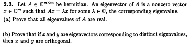
question: Do problem 2.3, page 15. For the latter, you may assume that the matrix is symmetric (i.e. \(A\) is real-values and \(A^{\prime }=A\)) and may examine there expressions of the form \(\left \langle Ax,y\right \rangle \)

solution

2.1 part a

Given: \(A\) is Hermitian, show that all the eigenvalues \(\lambda \) are real.

proof: Let \(x\) be an eigenvector of \(A\) with corresponding eigenvalue \(\lambda \), then \(Ax=\lambda x\), and taking the conjugate transpose of both sides \begin{align*} (Ax)^{\ast } & =(\lambda x)^{\ast }\\ x^{\ast }A^{\ast } & =\bar{\lambda }x^{\ast } \end{align*}

post multiply each side by \(x\) \begin{align*} x^{\ast }A^{\ast }x & =\bar{\lambda }x^{\ast }x\\ x^{\ast }(A^{\ast }x) & =\bar{\lambda }(x^{\ast }x) \end{align*}

And since \(A\) is Hermitian, then \(A=A^{\ast }\) and the above becomes \begin{align*} x^{\ast }(Ax) & =\bar{\lambda }(x^{\ast }x)\\ x^{\ast }(\lambda x) & =\bar{\lambda }(x^{\ast }x)\\ \lambda (x^{\ast }x) & =\bar{\lambda }(x^{\ast }x) \end{align*}

Since \(x\neq 0\) then the above implies \(\lambda =\bar{\lambda }\). This is only possible if \(\lambda \) is real. Hence all eiqenvalues of \(A\) must be real.

2.2 part b

Given: \(x,y\) are eigenvectors corresponding to distinct eigevalues. show that \(x,y\) are orthogonal

proof: Let \(\lambda _{x}\) be the eigenvalue corresponding to \(x\) and let \(\lambda _{y}\) be the eigenvalue corresponding to \(y\) and let. Then \begin{align*} Ax & =\lambda _{x}x\\ Ay & =\lambda _{y}y \end{align*}

Hence from the first equation above, taking the complex conjugate \begin{align*} (Ax)^{\ast } & =(\lambda _{x}x)^{\ast }\\ x^{\ast }A^{\ast } & =\bar{\lambda }_{x}x^{\ast } \end{align*}

post multiply each side of the above by \(y\) gives \begin{align*} x^{\ast }A^{\ast }y & =\bar{\lambda }_{x}x^{\ast }y\\ x^{\ast }(A^{\ast }y) & =\bar{\lambda }_{x}x^{\ast }y\\ x^{\ast }(Ay) & =\bar{\lambda }_{x}x^{\ast }y\\ x^{\ast }(\lambda _{y}y) & =\bar{\lambda }_{x}x^{\ast }y\\ \lambda _{y}x^{\ast }y & =\bar{\lambda }_{x}x^{\ast }y \end{align*}

But \(\bar{\lambda }_{x}=\lambda _{x}\) from part a, hence \(\lambda _{y}x^{\ast }y=\lambda _{x}x^{\ast }y\) and since \(\lambda _{y}\neq \lambda _{x}\) since we assumed all eigenvalues are distinct, then the above implies that \[ x^{\ast }y=0 \] which means that \(\left \langle x,y\right \rangle =0\) which implies \(x\) and \(y\) are orthogonal.

3 problem 2

solution

3.1 part (a)

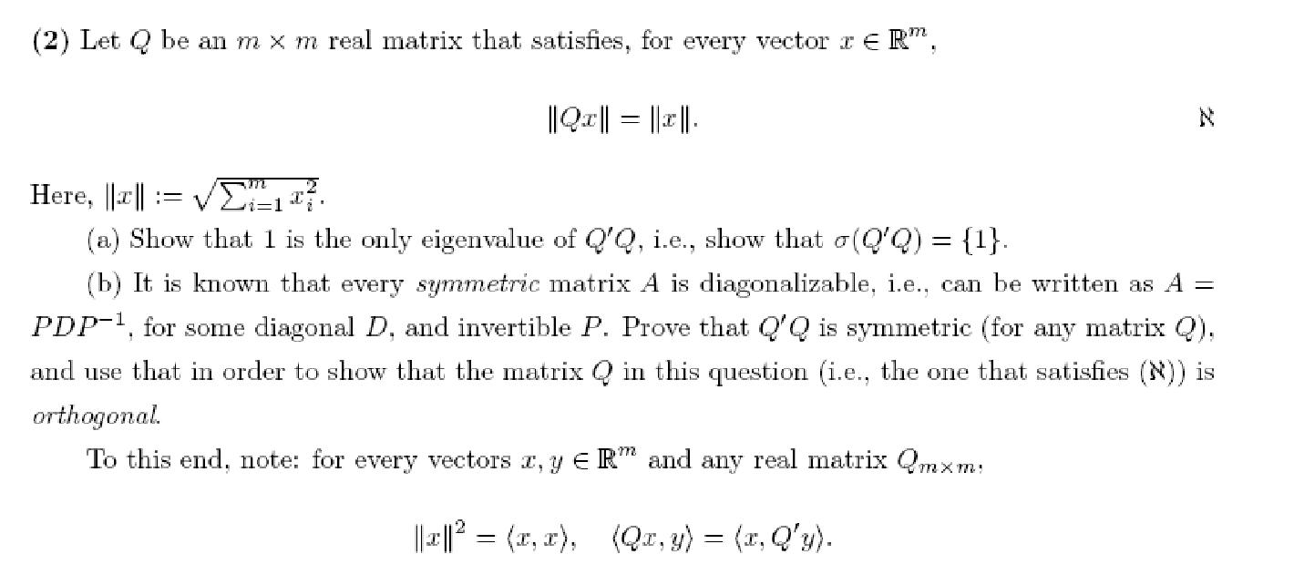
given \(\left \Vert Qx\right \Vert =\left \Vert x\right \Vert \) shown that \(1\) is only eigenvalue of \(Q^{T}Q\).

By definition \begin{align*} \left \Vert Qx\right \Vert & =\left ( Qx\right ) ^{T}\left ( Qx\right ) \\ & =\left ( x^{T}Q^{T}\right ) \left ( Qx\right ) \\ & =x^{T}\left ( Q^{T}Q\right ) x \end{align*}

But we are told that \(\left \Vert Qx\right \Vert =\left \Vert x\right \Vert \) and since \(\left \Vert x\right \Vert =x^{T}x\,\) we can write

\begin{align*} x^{T}\left ( Q^{T}Q\right ) x & =\left \Vert x\right \Vert \\ & =x^{T}x \end{align*}

Therefore, for the LHS above to be equal to the RHS, it must be that \(Q^{T}Q=I\) where \(I\) is the identity matrix. But the only eigenvalue of \(I\) is \(1\), since \(Iv=v\) for any \(v\). Therefore \(1\) is the only eigenvalue of \(Q^{T}Q\) which can be written as \(\sigma \left \{ Q^{T}Q\right \} =\left \{ 1\right \} \)

3.2 part (b)

We need to show that \(Q^{T}Q\) is symmetric for any matrix \(Q\). By definition, a matrix \(A\) is symmetric if \(A^{T}=A\). But

\[ \left ( Q^{T}Q\right ) ^{T}=Q^{T}\left ( Q^{T}\right ) ^{T}\]

But \(\left ( Q^{T}\right ) ^{T}=Q\) for any matrix \(Q\), hence

\[ \left ( Q^{T}Q\right ) ^{T}=Q^{T}Q \]

We have shown that \(A^{T}=A\), where \(A\) happened to be \(Q^{T}Q\) in this case. Hence \(Q^{T}Q\) is symmetric for any \(Q\).

Now we need to use this property to show that \(\left \Vert Qx\right \Vert =\left \Vert x\right \Vert \) implies that \(Q\) is orthogonal as well.

A matrix is orthogonal if each one of its columns (or rows) is orthogonal to each other column (or row). In addition, the normal of each column (or row) is one.

The first property above means that \(\left \langle q_{i},q_{j}\right \rangle =\delta _{ij}\) where \(\delta _{ij}=1\) if \(i=j\) and zero otherwise and where \(q_{i}\) means the \(i^{th}\) column (or row) of \(Q\) and \(q_{j}\) means the \(j^{th}\) column (or row) of \(Q\). But from part (a) above, we showed that \(Q^{T}Q=I\) which is the same as saying that \(\left \langle q_{i}^{T},q_{j}\right \rangle =\delta _{ij}\). Hence \(Q\) meets the first propery of orthogonality. Now we need to show that the norm of each column (or row) of \(Q=1\).

Since \(\left \Vert q_{i}\right \Vert =\sqrt{q_{i}^{T}q_{i}}=\sqrt{\delta _{ii}}=\sqrt{1}=1\), then the norm is \(1\). Hence both properties are satisfied. Hence \(Q\) is unitary matrix (or orthogonal).

4 Problem 3

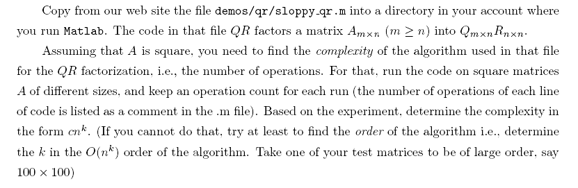
Solution