Simple detailed worked examples using Gaussian Quadrature method
Nasser Abbasi
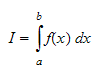
We seek to find a numerical value for the definite integral of a real valued
function of a real variable over a specific range. In other words, to evaluate
Geometrically, this integral represents the area under
 from
from
 to
to

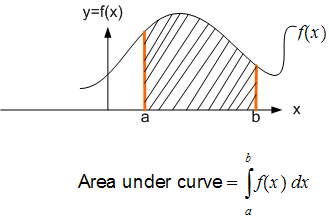
The following are few detailed step-by-step examples showing how to use Gaussian Quadrature (GQ) to solve this problem.
Few points to remember about GQ.
There are different versions of GQ depending on the basis polynomials it uses
which in turns determines the location of the integration points. We will only
use GQ based on Legendre polynomials. The integration points (called
 )
are the roots of the Legendre polynomials.
)
are the roots of the Legendre polynomials.
GQ gives an exact answer when the function to be integrated is a polynomial of
order
 where
where
 is the number of integration points.
Since Legendre polynomials are defined over
![$[-1,1]$](graphics/numIntegration__9.png) ,
we need to map the range of the function to be integrated to be
,
we need to map the range of the function to be integrated to be
![$[-1,1]$](graphics/numIntegration__10.png) .
The actual integration is performed over
.
The actual integration is performed over
![$[-1,1]$](graphics/numIntegration__11.png) but the values are mapped back to the original range using a transformation
rule. This diagram illustrates this.
but the values are mapped back to the original range using a transformation
rule. This diagram illustrates this.
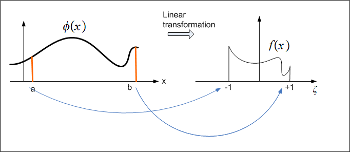
See appendix to see how the transformation rule is derived.
To be consistent, we follow the book notations and call the user function to
be integrated as
 and the mapped function as
 .
.
Using GQ, we need to have access to a lookup table to obtain the values of the
weights (called Multipliers or
 in the book) and the integration points
 .
For each different value of
.
For each different value of
 (the numbers of integration points, also called the order of GQ), there will
be a specific set of values
(the numbers of integration points, also called the order of GQ), there will
be a specific set of values
 and
and
 to use. Once we have
 and
and
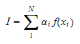
 then the value of the integral is
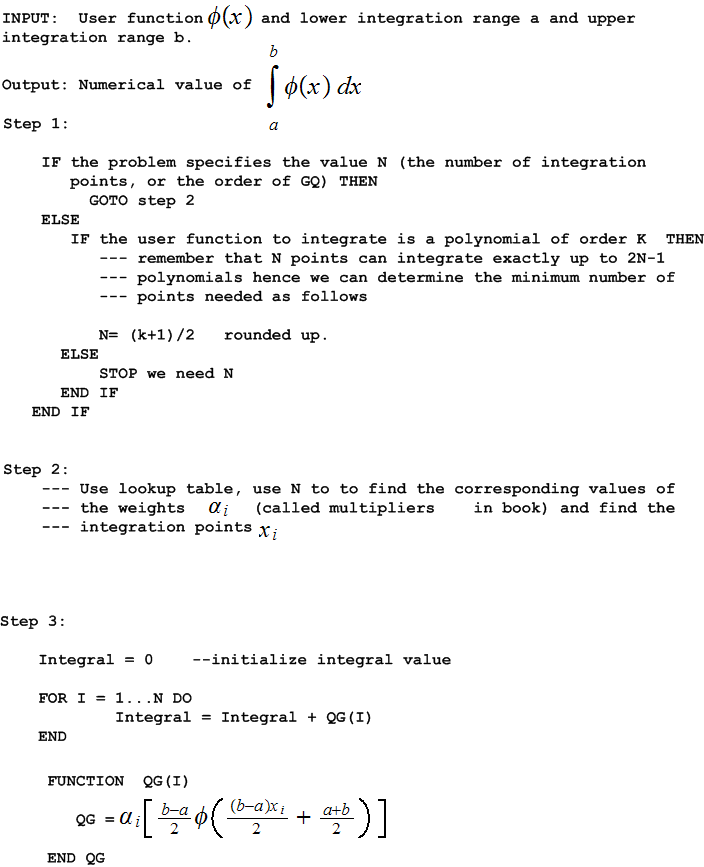
This is an overview of the GQ algorithm. Next we will work out few examples to illustrate.
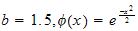
Evaluate
 ,
Use
,
Use

We see that
 ,
,
Answer
step 1:
 is given, go to step 2.
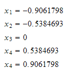
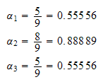
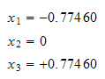
step 2: From lookup we see that
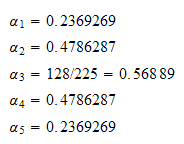
And
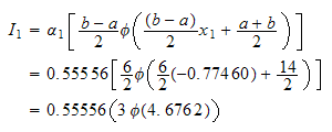
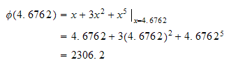
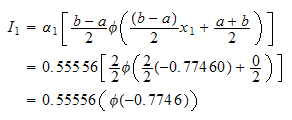
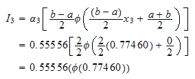
step 3: Evaluate the integral
LOOP over all the points from left to right.
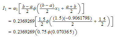
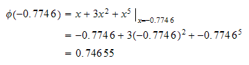
But
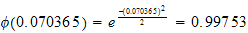
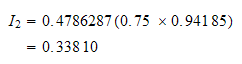
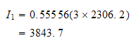
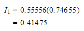
Hence
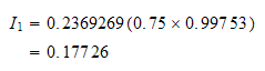
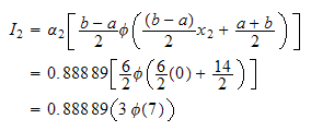
Do the next point:
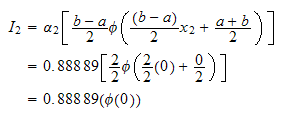
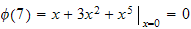
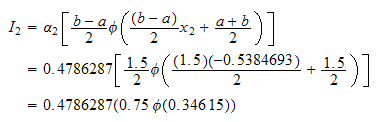 But
But
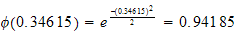
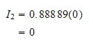
Hence
Do the next point
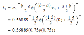
But
Hence
Do the next point
 But
But
Hence
Do the next point
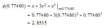
 But
But
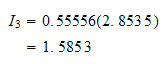
Hence
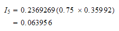
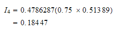
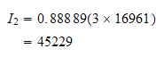
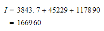
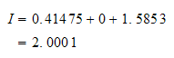
No more points. Add to obtain the final answer
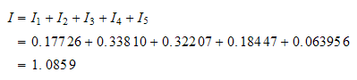
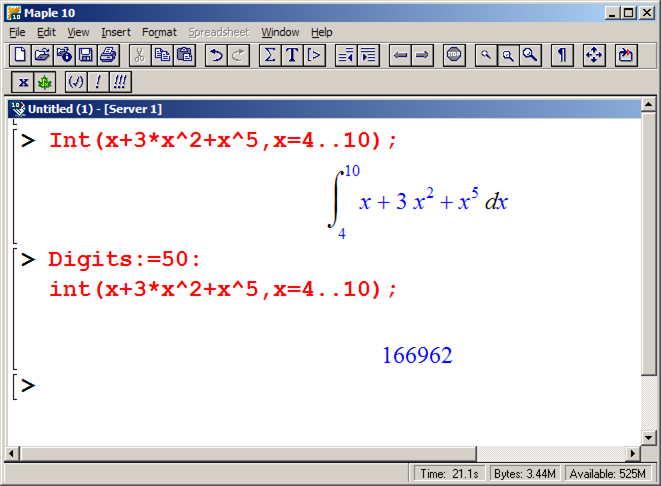
To verify, use say Maple:
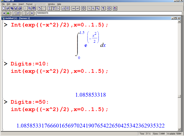
Evaluate
We see that
 ,
,
Answer:
step 1:
 is not given. But since polynomial, we can determine minimum

Order of polynomial is
 hence we need

step 2: From lookup we see that

And

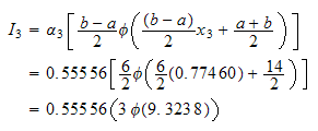
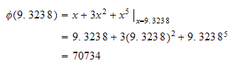
step 3: Evaluate the integral
LOOP over all the points from left to right.
But
Hence
 Do next point
But

Hence
Do next point
But
Hence
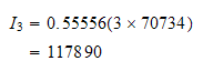
Hence the answer is
Verify
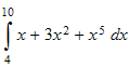
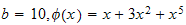
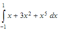
Evaluate
We see that
 ,
,
Answer:
step 1:
 is not given. But since polynomial, we can determine minimum

Order of polynomial is
 hence we need

step 2: From lookup we see that
And
step 3: Evaluate the integral
LOOP over all the points from left to right.
But
Hence
 Do next point
But
Hence
Do next point
But
Hence
Hence the answer is
An easy way to find how the function changes when we change the range is to
align the ranges over each others and take the ratio between them as the scale
factor. This diagram shows this for a general case where we map
 defined over
![$[a,b]$](graphics/numIntegration__88.png) to a new range defined over
to a new range defined over
![$[c_{1},c_{2}]$](graphics/numIntegration__89.png)
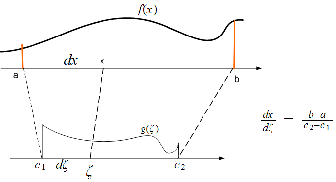
 We
see from the diagram that
We
see from the diagram that

But
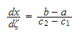
The above is called the Jacobian of the transformation.
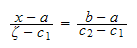
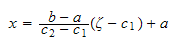
Now, From the diagram we see that

and

Hence (1) becomes
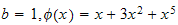
For the specific case when
 and
and
 the above expressions become
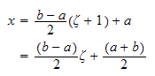
Which is the mapping used in the Gaussian Quadrature method.
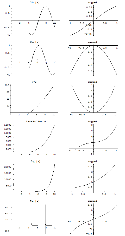
It interesting to see the effect of this transformation on the shape of some
functions. Below I plotted some functions under this transformation. The left
plots are the original functions plotted over some range, in this case
![$[4,10]$](graphics/numIntegration__101.png) and the left side plots show the new shape (the function
and the left side plots show the new shape (the function
 )
over the new range
)
over the new range
![$[-1,1]$](graphics/numIntegration__103.png)