Midterm MAE185, Spring 2006. Take home problem solution.

This solves the take home problem for midterm MAE185.

The problem is the last problem here [PDF]

Write the fortran code, then compile it and run it as follows

$ g95 sol.f90

$./a.exe > output.txt

You only need to show the independent variable t vs. the first derivative f’(t). But in the above I printed all the state variables. The format is as follows

T F F’ F’’

So there are 4 columns. I used double precision for all the variables, but single precision will also work if you use the correct epsilon for the correct precision.

SOURCE CODE [sol.f95 , sol.f95.txt]

OUTOUT [output.txt]

Windows executable [sol.exe]

PLOTS. Used Matlab to display the solution as follows

>> A=load('output.txt');

>> size(A)

ans =

1361 4

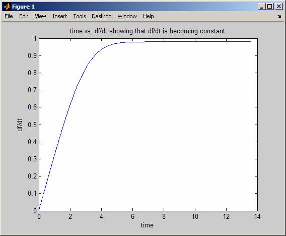
>> plot(A(:,1),A(:,3))

>> title('time vs. df/dt showing that df/dt is becoming constant')

>> xlabel('time'); ylabel('df/dt');

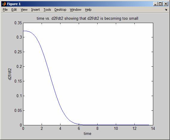
Here is a plot of time vs f’’, showing that f’’ is getting too small as f’ is becoming constant

>> plot(A(:,1),A(:,4))

>> xlabel('time'); ylabel('d2f/dt2');

>> title('time vs. d2f/dt2 showing that d2f/dt2 is becoming too small')

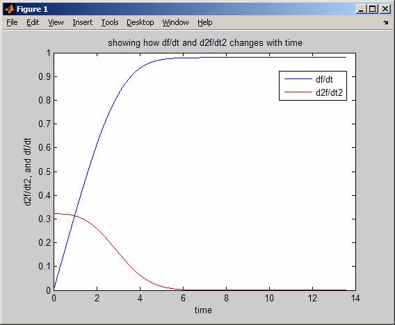
Here are the 2 plots on same figure

>> close all

>> plot(A(:,1),A(:,3))

>> hold on

>> plot(A(:,1),A(:,4),'r')

>> xlabel('time'); ylabel('d2f/dt2, and df/dt');

>> title(' showing how df/dt and d2f/dt2 changes with time')

>> legend('df/dt','d2f/dt2')

>>