![$[0,L]$](graphics/MAE200B_HW1_prob_1__1.png) by separation of variables.
by separation of variables.
 for
for
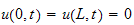
 with the boundary conditions
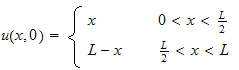
 and the initial conditions specified by the function
HW 1, MAE 200B.
Problem 1
by Nasser Abbasi
UCI, Winter 2006.
Question
Solve the following IBVP for the 1D heat conduction problem over the interval
by separation of variables.
for
with the boundary conditions
and the initial conditions specified by the function
Solution
Assume the solution is of the form
 where
where
 and
and
 are functions which are independent of each others, i.e.
 is a function of
 only and
 is a function of
 only.
only.
Substitute this form in the PDE above we obtain
 ,
and now divide both sides by
,
and now divide both sides by
 we obtain
 .
.
Since the left hand side is a function which depends on time only and the
right hand side is a function which depends on
 only and both are equal, hence they both must equal to a constant, say
 .
Hence we obtain the following 2 ODE's to solve:
.
Hence we obtain the following 2 ODE's to solve:
 or
or

and
 or
or

Start by solving the spatial ODE. Assume the solution to
 is of the form
 ,
and substitute this back in the ODE we obtain the characteristic equation
,
and substitute this back in the ODE we obtain the characteristic equation
 ,
and divide both side by
,
and divide both side by
 we get
 ,
hence the solution can be written as
,
hence the solution can be written as
So one general solution to
 is a sum of scaled version of these 2 basic solution, i.e.
case (1):

Apply the spatial B.C. to the above solution to determine
 and
and
 ,
we get from the B.C. at
,
we get from the B.C. at
 the equation
 and from the B.C. at
 we obtain the equation
 .
.
Hence
 and substitute this in the second equation above, we obtain
 .
But for a non-trivial solution,
.
But for a non-trivial solution,
 hence this means that
 or
or
 and since we assumed
 this implies that
 for
some positive
for
some positive
 but this is not possible unless
 ,
hence
,
hence
 only gives a trivial solution
 or
or
 .
.
case(2):

When
 the
ODE is
the
ODE is
 which has the solution
 ,
and when we apply the B.C. we obtain
,
and when we apply the B.C. we obtain
 and
and
 or
or
 ,
hence this results also in a trivial solution
,
hence this results also in a trivial solution

case(3)

Let
 for some constant
 ,
hence eq (1) above can be written as
,
hence eq (1) above can be written as
 which can be rewritten (using Euler relations
 and
and
 )
as
)
as
Apply the B.C. at
 we obtain
 hence
hence
 ,
and now apply the B.C. at
,
and now apply the B.C. at
 we obtain
 and
to avoid a trivial solution
and
to avoid a trivial solution
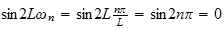
 we must have that
 or
or
 or
or
 for
for

Hence the solution for the spatial ODE is
Where
 for
for
 and we assumed the constant

Now we need to find solution to the time ODE. For each
 we have a solution.
Since
we have a solution.
Since ,
assume solution is of the form
,
assume solution is of the form
 hence the characteristic equation leads to
 hence the solution is
 but
but
 hence
hence
 or
or
By choosing

Hence the overall solution is
By principle of superposition, the general solution is a scaled sum of these
solutions. where the scaling parameter depends on
 which
we call
which
we call
 i.e.
i.e.
Now apply the initial condition
 ,
from eq (2) above we obtain that
,
from eq (2) above we obtain that
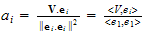
Compare this an expression where we write a vector in terms of its basis as in
 . To find the vector components
 we apply the inner product as follows:
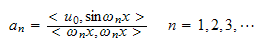
 hence using similar idea, we apply this to find the components
 by considering in this case the vector
 as being the function
 and it is being decomposed to its basis
 as what we do normally in fourier series expansion. Hence we now can find
 by writing
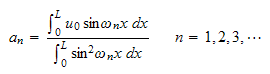
 and take the inner product over
![$[0,L]$](graphics/MAE200B_HW1_prob_1__102.png) we obtain
we obtain
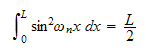
But

But
 hence we get that
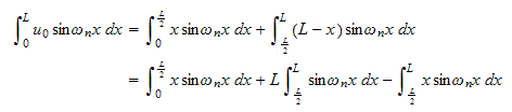
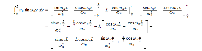
Now to evaluate
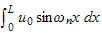 , we rewrite as sum of 2 integrals for each of the ranges of the initial
condition as follows
, we rewrite as sum of 2 integrals for each of the ranges of the initial
condition as follows
But
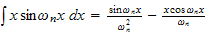 by integration by parts. Apply this to the above we obtain
But
 hence above
becomes
hence above
becomes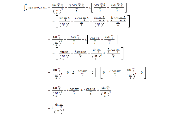
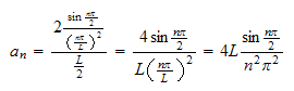
Hence
Try for few
 values
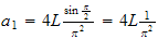
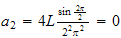
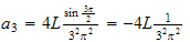
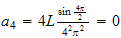
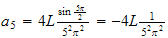
Hence
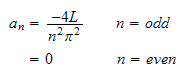
Since
 for even
 ,
we only need to sum over odd values of
,
we only need to sum over odd values of

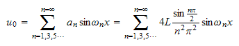
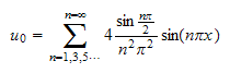
Hence
When
 and
and

 And
the general solution is from eq (2)
:
And
the general solution is from eq (2)
: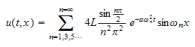
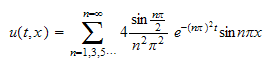
Now consider the case when
 and
and
 hence the solution is
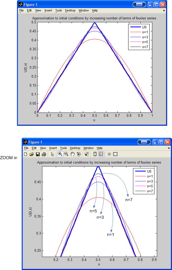
The following is a plot of the initial condition
 and the approximation to it as given by eq(4) above by using trying different
values of
and the approximation to it as given by eq(4) above by using trying different
values of
 .
I tried for
.
I tried for
 ,
we see that as
,
we see that as
 increases, the summation approximation becomes closer and closer to the
initial condition function
increases, the summation approximation becomes closer and closer to the
initial condition function
 as expected from Fourier series expansion.
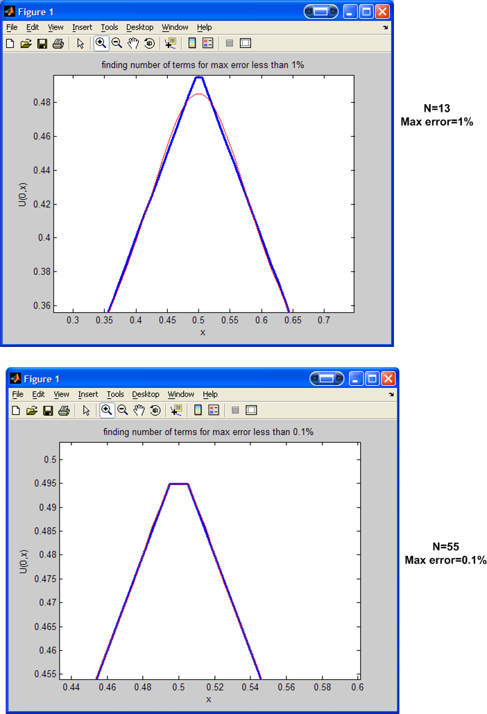
To find the number of terms we need so that the approximation is consider
'good', I will find, for each
 ,
the maximum of the error that occurs between the function
,
the maximum of the error that occurs between the function
 and the function represented by the sum.
Will stop when the maximum error is less than some tolerance, say
 or
or
 .
The following is the Matlab code and the plot result and the final
.
The following is the Matlab code and the plot result and the final
 was found to be.
The result shows that if we want maximum error to be less than
 then
then
 ,
and for maximum error to be less than
,
and for maximum error to be less than
 then
then

I will use
 since this make the approximation almost the same as
 .
.
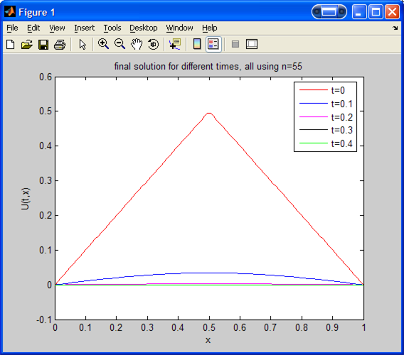
Now use this
 to find the final solution given by equation (5) above
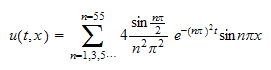
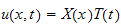
The following is the plot of
 for different
 values.
The following is another plot but using smaller time increments of 0.01
seconds, up to