LAB #7 report. MAE 106. UCI. Winter 2005

Nasser Abbasi, LAB time: Friday 2/25/2005 10 AM

Answer 1.

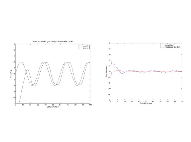
I have tried a number of runs with different proportional and derivative gain constants running at Hz. This plot below shows few of the tests I've run, and below them the one I think achieved the best tracking.

Derivative gain=0.4

Proportional gain=0.4

Answer 2

First I need to derive the transfer function. I can decide to control the speed of the motor shaft, or its angular position. I need to decide on this since this affect what the transfer function will be. i.e. wither I will select the position or the speed to be the output. In both cases I will take the motor voltage supply as the input.

I selected to use position as the controller variable.

First, I show the model of the motor itself, then the block diagram. Next I show the block diagram with a delay element added in the feedforward path, and the compare the transfer functions with and without delay and show that with delay, it is possible for the output to become unstable.

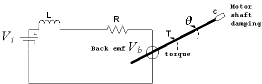
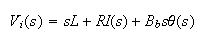
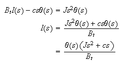
From the diagram below, using Kirchoff law around the motor circle, we get

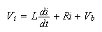
Take Laplace transform we get

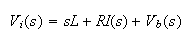
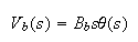
Now, we know that the backemf voltage produced is proportional to the angular speed of the shaft. Let this proportionality constant be called then we write

Take Laplace transform of the above, we get

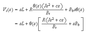
Substitute equation (2) into (1) we get

Now consider the dynamic equation for the motor shaft, we get

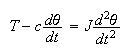
Where is the moment of inertial of the motor shaft around its axis of rotation. Take Laplace transform of the above we get

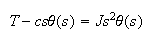
We also know that the torque produced is proportional to the current in the motor. Lets call the proportionality constant hence we write

Take Laplace transform of (5) we get

Substitute (6) into (4) we get

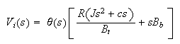
Now substitute (7) into (3) we get

Now is usually very small compare to so equation (8) can be written as

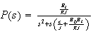
Hence the transfer function between and is

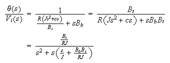
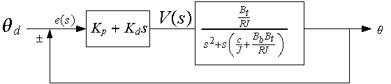
This transfer function is in the standard form. It is a second order system. The above is the transfer function of the plant itself. Now I put the above into the loopback block diagram, assuming the controller we used is PD controller of the form we get this

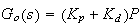
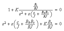
Now we do block simplification to obtain the closed loop transfer function. Let , hence the feedforward transfer function is hence the closed loop transfer function is

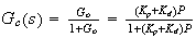
Let then we write

The charaterstic equation is . The closed loop poles are the roots of this equation.

Replace above to be able to solve for the roots, we get

the roots are

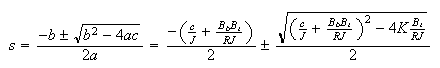
We see from the above, that independent of the values under the sign, the system will have its poles in the left hand side. This is because the quantity is positive.

Hence the system is always stable no matter how large the gain is.

Now let see what happens when we add the effect of Labjack into the system, model this effect as a time delay, which in the Laplace transform becomes where is the time it takes Labjack to sample one data point, i.e. is the sampling period. Hence now the block diagram becomes

Where I wrote as the output from the labjack. (delayed voltage).

Now, since

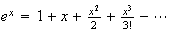
Then

Now for very small all terms with for can be ignored. Hence we get an approximation

Hence the above system becomes

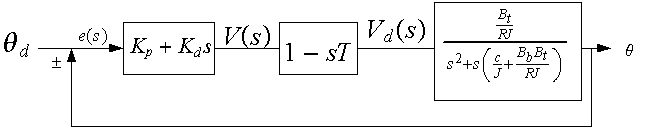
Now obtain the closed loop transfer function.

The open loop transfer function is

As before, let , hence we get

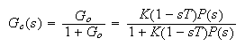
Then the closed loop transfer function is

The characteristic equation is

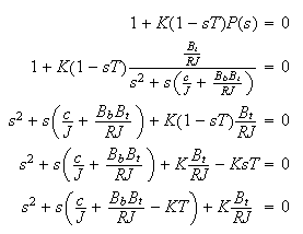
The roots of this equation (i.e. the poles of the closed loop) now can be found as

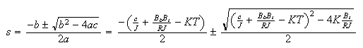
Now we clearly see the effect of the delay of the closed loop poles.

We see that the real part of the pole can occur at the positive side of the s plane, and this will happen when 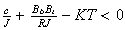or when

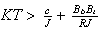
hence we see that as is increased, the closed loop pole will move to the right until it will cross the imaginary axes making the system unstable. In addition, for a fixed gain , as is increased the system can become stable. An increase in implies that the sampling frequency becomes smaller, since .

This is what we are asked to show.