of its final value.
LAB #2 report. MAE 106. UCI. Winter 2005
Nasser Abbasi, LAB time: Thursday 1/20/2005 6 PM
Explain time constant: This is the time the output will take to reach
of its final value.
Cut-off frequency is the frequency at which the output amplitude (Such as
voltage) is
 of the input. This corresponds to a drop of
 from the input. It is also the frequency at which the output power is
 that of the input. This frequency is usually taken as the boundary frequency
between the highpass region and the low pass region of the frequency response
plot.
that of the input. This frequency is usually taken as the boundary frequency
between the highpass region and the low pass region of the frequency response
plot.
A heavy object has large inertia. Which means it will take time for it to accelerate when subjected to the same force as compared to an object of low mass. When the force fluctuates very quickly, the object will be slow to react due to its high mass, and by the time it starts to move in response to the force, the force will change its direction quickly, and the object will have to start to reverse its direction again in the direction of the force, and will again be slow in doing this new movement. So this mean the object will have a small motion amplitude of the same frequency as the input force. This is a low pass filter.
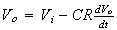
I collected the data using LabJack. This below shows the first few lines of the text file collected:
Now I wrote a small script to plot the data and the theoretical response
 on the same plot. this is the result. I normalized both amplitudes to 1.
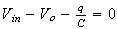
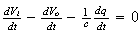
For the circuit in figure 1, the ODE is
 .
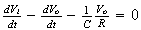
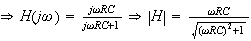
Take Laplace transform, we get
.
Take Laplace transform, we get


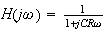
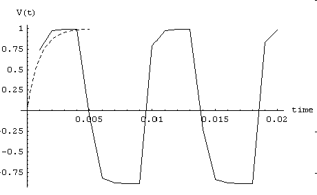
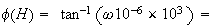
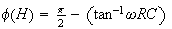
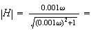
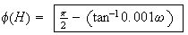
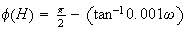
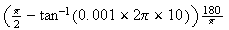
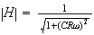 and phase is
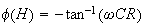
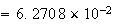
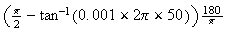
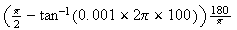
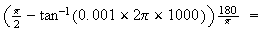
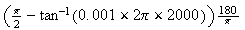
Hence for
 ,
and
,
and
 we get
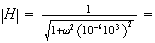


and
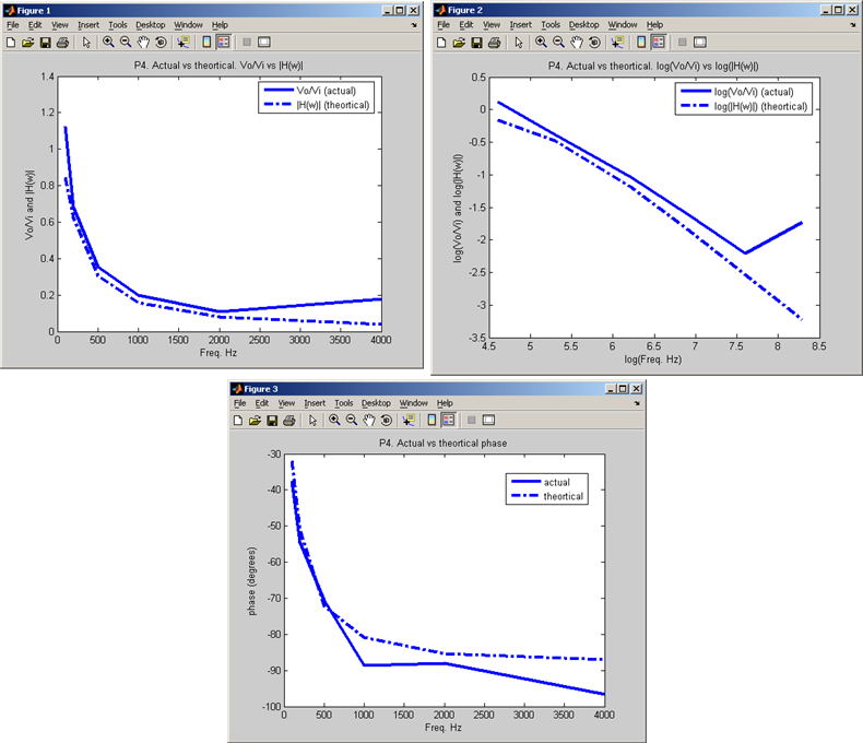
The following is the data collected for P4, and the theoretical data based on above Laplace transform. This is a low pass filter.
| Input Freq. (Hz) |  input input |
 output
 |
 |
 |

 (degrees) (degrees) |
| 100 | 590 mV | 662 mV | 1.04 ms | 10 ms | 
 -
- |
| 200 | 1.7 V | 1.156 V | 740
 |
4.9 ms |  -
- |
| 500 | 1.59 V | 562 mV | 390
 |
1.99 ms | 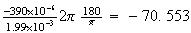 |
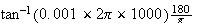
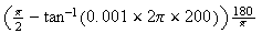
| 1 K | 1.562 V | 312 mV | 244
 |
990
 |
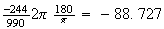 |
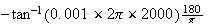
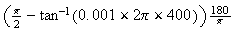
| 2 K | 1.56 V | 171 mV | 126
 |
515
 |
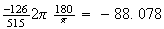 |
| 4 K | 2.8 V | 500 mV | 65
 |
242
 |
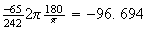 |
Theortical:
| Input Freq. (Hz) |  |
 rees rees |
| 100 | 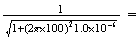
 |
- |
| 200 | 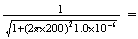
 |
-
 |
| 500 | 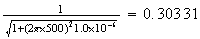 |
-
 -
- |
| 1 K | 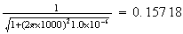 |
-
 |
| 2 K | 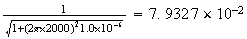 |
 |
| 4 K | 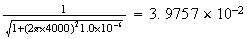 |
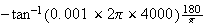
 |
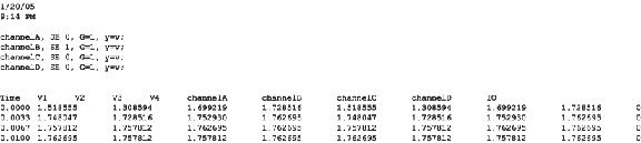
I now wrote a script to plot the needed plots as required by P4. This is the result. This shows that the amplitude plot involving the log is more clear and it shows the low pass filter, this is because when using the log scaling, the becomes straight lines.
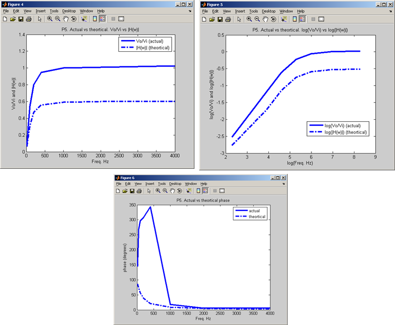
The following is the data collected for P5.
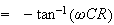
Since
 for the capacitor, and for the circuit in figure 3, we get
 .
Take derivative, we get
.
Take derivative, we get
 ,
but
,
but
 ,
hence ODE becomes
,
hence ODE becomes
 , take Laplace transform we get


Let
 ,
,
 and
and
Hence for
 ,
and
,
and
 we get


and
This is a high pass filter
| Input Freq. (Hz) |  output output |
 input
input |
 |
 |
 (degrees)
 |
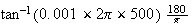
| 10 | 800 mV | 10 V | 38 ms | 97
 |
 |
| 50 | 3 V | 9.8 V | 15 ms | 20
 |


 |
| 100 | 5 V | 9.18 V | 8.24 ms | 10
 |


 |
| 200 | 6.6 V | 8.25 V | 4.34 ms | 5.07
 |


 |
| 400 | 7.3 V | 7.7 V | 2.4 ms | 2.52
 |
 |
| 1000 | 7.47 V | 7.47 V | 48
 |
989
 |


 |
| 2000 | 7.57 V | 7.47 V | 8
 |
500
 |


 |
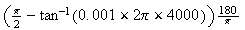
| 4000 | 7.5 V | 7.3 V | 4
 |
247
 |


 |
Theortical:
| Input Freq. (Hz) |  |
 |
| 10 | 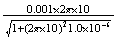
 |


 |
| 50 | 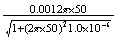 =
=
 |

 |
| 100 | 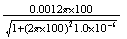 =
= |

 |
| 200 | 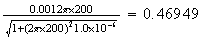 |

 |
| 400 | 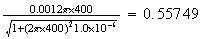 |
 |
| 1000 | 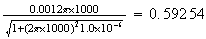 |
 |
| 2000 |  |

 |
| 4000 | 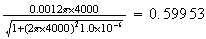 |

 |