Physics 229& 100 Homework #5
Name: Nasser Abbasi
1. Suppose that the profit your company makes is given by P=s m (3m+s)E^(-(2s +m)/40) , where s and m are the number of sales and manufacturing people, respectively. If the total number of people is equal to 50, how do you distribute the human resources to maximize your profit. By how much would profit increase if you hire an additional person? Do the problem two ways:
a) using Lagrange multipliers and FindRoot
The problem formulation is the following
Maximize the objective function P (which represents profit) subject to contraint g(x,m)=50, where in this problem g(x,m) is defined as x+m
If we consider a 3D space, where the z axis represents the profit, the x axis is s, and y axis is m, then we want to locate the point above the line s=50-m (marked as RED in the diagram, which is the constraint) where this point has the largest distance from the x-y plane, as shown in this diagram
![[Graphics:HTMLFiles/index_1.gif]](HTMLFiles/index_1.gif)
![Remove["Global`*"] ;](HTMLFiles/index_2.gif)

![RowBox[{RowBox[{f[s_, m_], :=, RowBox[{s, , m, , (3 m + s), , ^(-(2 s + m)/40), Cell[]}]}], ;}]](HTMLFiles/index_4.gif)
![g[s_, m_] := s + m - maxNumberOfPeople ;](HTMLFiles/index_5.gif)
![faux[s_, m_, λ_] := f[s, m] - λ g[s, m] ;](HTMLFiles/index_6.gif)
![eq1 = {D[faux[s, m, λ], m] == 0, D[faux[s, m, λ], s] == 0, D[faux[s, m, λ], λ] == 0} ;](HTMLFiles/index_7.gif)
![MatrixForm[%]](HTMLFiles/index_8.gif)

So we have 3 equations to solve for 3 unknowns,(s,m,λ).Since this is not a polynomials,we can't use Solve or NSolve,we need to find FindRoot[],but for that we need a guess.So lets make a plot of the profit to get a guess for s and m
![Plot3D[f[s, m], {s, 0, 50}, {m, 0, 50}, PlotLabel->"Profit vs m and s", AxesLabel→ {"s", "m", "profit"}] ;](HTMLFiles/index_10.gif)
![[Graphics:HTMLFiles/index_11.gif]](HTMLFiles/index_11.gif)
We see from the above that guess for s=15and m=35 looks promissing.Lets use that (what about λ?,I tried many different values,and it did not make a difference)
![sol = FindRoot[eq1, {{s, 15}, {m, 35}, {λ, 1}}]](HTMLFiles/index_12.gif)

Hence, since the solution must be an integer, we round the numbers
![s = Round[s/.sol]](HTMLFiles/index_14.gif)

![m = Round[m/.sol]](HTMLFiles/index_16.gif)

b) Using NMaximize
![Clear[s, m] ;](HTMLFiles/index_18.gif)
![NMaximize[{f[s, m], g[s, m] == 0}, {s, m}]](HTMLFiles/index_19.gif)

We see that the answer agrees with the method of the lagrange multiplier
2. Find the triangle of perimeter L with maximum area. A triangle is specified by three points in a plane. Put the first point at the origin, the second point along the x axis at {x1,0} , and the third point at {x2,y2}.
a) Write an expression for the area of the triangle in terms of x1,x2,y2 , neglecting the perimeter constraint.
![Remove["Global`*"] ;](HTMLFiles/index_21.gif)


b) What is the maximal area in terms of L?


![eq1 = {D[Aaux, x1] == 0, D[Aaux, x2] == 0, D[Aaux, y2] == 0, D[Aaux, λ] == 0} ;](HTMLFiles/index_28.gif)
![MatrixForm[eq1]](HTMLFiles/index_29.gif)
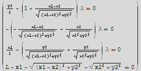
![sol = Solve[eq1, {x1, x2, y2, λ}] ;](HTMLFiles/index_31.gif)
![MatrixForm[sol]](HTMLFiles/index_32.gif)
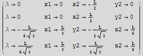


Hence maximum area in terms of L is the last case, which is
![areas[[4]]](HTMLFiles/index_40.gif)

3. Find the minimum distance between points in the intersection of
3x-4y+5z==8 and x+y-z==11
and points on the unit sphere. Do it 2 ways, and show that you get the same answer both ways:
a) using PseudoInverse and geometry ( utilizing the fact that the PseudoInverse solution to the simultaneous equations will have minimum length)
The constraint is the line of the interection. The objective function is the distance between this line and points on the unit sphere.
![Remove["Global`*"] ;](HTMLFiles/index_42.gif)
![Needs["Graphics`Shapes`"] ;](HTMLFiles/index_43.gif)
![Needs["Graphics`Colors`"] ;](HTMLFiles/index_44.gif)
![plan1[x_, y_] := 1/5 (8 + 4 y - 3 x) ;](HTMLFiles/index_45.gif)
![plan2[x_, y_] := 11 - y - x ;](HTMLFiles/index_46.gif)
![p1 = Plot3D[plan1[x, y], {x, -4, 16}, {y, -4, 16}, PlotPoints→50, ViewPoint→ {-2, -2.4, 2.}, DisplayFunction→Identity] ;](HTMLFiles/index_47.gif)
![p2 = Plot3D[plan2[x, y], {x, -4, 16}, {y, -4, 16}, PlotPoints→30, ViewPoint→ {-2, -2.4, 2.}, DisplayFunction→Identity] ;](HTMLFiles/index_48.gif)
![Show[{p1, p2}, DisplayFunction→$DisplayFunction] ;](HTMLFiles/index_49.gif)
![[Graphics:HTMLFiles/index_50.gif]](HTMLFiles/index_50.gif)

![r = 5 ; (*I enlarge the sphere just to be able to see it*)p0 = WireFrame[Graphics3D[Sphere[r, 15, 15], DisplayFunction→Identity]] ;](HTMLFiles/index_52.gif)
![Show[{p1, p2, p0}, DisplayFunction→$DisplayFunction] ;](HTMLFiles/index_53.gif)
![[Graphics:HTMLFiles/index_54.gif]](HTMLFiles/index_54.gif)
Now use PsudoInverse to find the point on the line of the intersection of the 2 planes where the point is closes to the origin
![Clear[x, y, z] ;](HTMLFiles/index_55.gif)
![Needs["LinearAlgebra`MatrixManipulation`"] ;](HTMLFiles/index_56.gif)


![{A, b} = LinearEquationsToMatrices[{eq1, eq2}, {x, y, z}] ; MatrixForm[A]](HTMLFiles/index_59.gif)

![MatrixForm[b]](HTMLFiles/index_61.gif)

![{x, y, z} = PseudoInverse[A] . b//N](HTMLFiles/index_63.gif)

![distaceFromOrigin = Sqrt[x^2 + y^2 + z^2]](HTMLFiles/index_65.gif)

The above is the distance to the origin. Hence the distance to the surface of the sphere is


b) using Lagrange multipliers.
Let xc,yc,zc represent coordinates of a point on the sphere. Let xp,yp,zp represent coordinates of a point on the surafces. Now setup the object function and the constrains and the auxilary function.
![Remove["Global`*"] ;](HTMLFiles/index_69.gif)


![eq = Thread[{D[fAux, xc], D[fAux, yc], D[fAux, zc], D[fAux, xp], D[fAux, yp], D[fAux, zp]} == 0]](HTMLFiles/index_81.gif)
![MatrixForm[eq]](HTMLFiles/index_82.gif)


![maxeqs = Join[eq, {g1 == 0, g2 == 0, g3 == 0}] ;](HTMLFiles/index_85.gif)
![MatrixForm[maxeqs]](HTMLFiles/index_86.gif)
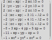
![sol = NSolve[maxeqs, {xc, yc, zc, xp, yp, zp, λ1, λ2, λ3}] ;](HTMLFiles/index_88.gif)
![MatrixForm[%]](HTMLFiles/index_89.gif)


![Min[minDistance1, minDistance2]](HTMLFiles/index_95.gif)

We see that the solution agrees with part(a).
4 a) The Wronskian of a set of functions { [x],
[x],  [x]...,
  [x] } is defined as
det(
). Write a function wronski[funcs_List, var_] that will compute the Wronskian of any set of functions. Use it to compute the Wronskian of { ,
, , Sin[x]} and of {
 ,
, , Sinh[x]}
![Remove["Global`*"] ;](HTMLFiles/index_113.gif)
![wronski[funcs_List, var_] := Det[NestList[D[#, var] &, funcs, Length[funcs] - 1]] ;](HTMLFiles/index_114.gif)
![wronski[{E^x, E^-x, Sin[x]}, x]](HTMLFiles/index_115.gif)
![4 Sin[x]](HTMLFiles/index_116.gif)
![wronski[{E^x, E^-x, Sinh[x]}, x]](HTMLFiles/index_117.gif)

b) One of the uses of the Wronskian is to determine if a set of functions is linearly independent. Recall that two vectors v1 and v2 are independent if A v1+B v2=0 implies that A and B are zero. Similarly, if the only solution to A y1[x]+B y2[x]=0 ( for all x) is the trivial one {A->0,B->0}, y1 and y2 are independent functions. Note that if A y1[x]+B y2[x]=0, then by taking a derivative, we conclude that A y1' [x]+B y2' [x] must also vanish. Show that the condition for independence is that the Wronskian of y1 and y2 does not vanish for all x.
sketch of proof:
Assume that  and
and  are L.d. and show that this implies that W=0
Then assume that W=0 and show that this implies that  and
and  are L.d.
Hence if W /= 0, then this must imply that  and
and  are L.I.
Start of proof:
Assume  and
and  are L.d then we can write
 =
= 

where  is some constant
Then
 =
= 

Now W=(
)
=(
)
Hence the determinant of W is


 '-
'-

 ' = 0
' = 0
Now for the second part. Assume that det(W)=0, then this means

 '-
'-
 ' = 0 -----------------(1)
But differentiation itself is a linear operation, hence we can write
 =
=
 ------(2)
and
 =
=
 -----(3)
Where  and
and  are some arbitrary constanst which are unrelated.
Substitute the above 2 equations into equation (1) we obtain


 -
-

 = 0
= 0
Divide by  we obtain

 =
=

which means  =
= (else we have
  =0 everywhere)
Since  =
= , then if we divide equation (2) by (3) we obtain
 =
=
Which implies that  is L.d. to
  . This complete the second part of the proof.
Hence if det(W)/=0, then  must be L.I. to
This completes the proof.
c) Consider a second order DE with coefficients that are not necessarily constant:
y''[x]+p1[x] y'[x]+p0[x] y[x]=0. Let y1[x] and y2[x] be two solutions to this equation. Let W be the Wronskian of the two solutions. Show that  =-p1[x] W[x]. If p1[x] is constant, show that if W is non zero for any x, it will be non zero for all x.
I will just write everything without [x] next to it for ease of reading.
W=det (
)=y1 y2'-y2 y1'
Hence  =y1' y2' + y1 y2''- y2' y1'- y2 y1'' ------(1)
Since y1[x] is a solution, then
y1''=-p1 y1' -p0 y1
Similarly, since y2[x] is a solution then
y2''=-p1 y2' -p0 y2
Substitute the above 2 equations into (1) we obtain
 =y1' y2' + y1 (-p1 y2' -p0 y2)- y2' y1'- y2 (-p1 y1' -p0 y1)
 =y1' y2' - y1 p1 y2' -y1 p0 y2- y2' y1'+ y2 p1 y1' + y2 p0 y1
 =y1' y2' - y1 p1 y2' - y2' y1'+ y2 p1 y1'
 =- p1 (y1 y2' - y2 y1' )
But the last term above is W, hence
 =- p1[x] W[x]
Which is what we are asked to show.
Last part. If p1[x] is constant, say m then the above is  =mW[x] which has the solution of W(x)=n
  where n is some other constant.
Hence we see that if we can find one x where W(x) is not zero, then this implies that the constant n is not zero (since the exponential term is not zero unless x=-∞). So, if n≠0 and since the exponential term is not zero then W(x) can not be zero for any other x.
5. Write a function waveEq[f_] which computes the wave operator  f-
f-
 in spherical coordinates f[r,θ,φ,t] ( use the VectorAnalysis Add-on package). The wave operator is identically zero if f satisfies the wave equation. Use it to show that
  is a solution for certain values of the scalar k.
![Remove["Global`*"] ;](HTMLFiles/index_195.gif)
![Needs["Calculus`VectorAnalysis`"]](HTMLFiles/index_196.gif)
![Needs["MMHTools`DForm`"]](HTMLFiles/index_197.gif)
![SetCoordinates[Spherical[r, θ, φ]]](HTMLFiles/index_198.gif)
![Spherical[r, θ, φ]](HTMLFiles/index_199.gif)
![waveEq[f_] := Laplacian[f] - 1/c^2D[f, {t, 2}]](HTMLFiles/index_200.gif)
![sol = waveEq[f[r, θ, φ, t]]](HTMLFiles/index_201.gif)

![DForm[sol]](HTMLFiles/index_203.gif)


![sol = waveEq[g]](HTMLFiles/index_206.gif)

![sol = Simplify[sol]](HTMLFiles/index_208.gif)

![Reduce[sol == 0, k]](HTMLFiles/index_210.gif)

We see that the solution is zero form specific values of k, which are +- frequency/speed of light
6. A plane wave polarized in the x direction and propagating in the z direction has an electric field E1={ex, 0, 0} , where ex is the magnitude of the field and k is a constant vector k={0, 0, km}. According to Maxwell's equations, this wave has a magnetic field associated with it which obeys the equation ∇×E=-
 .
.
a) Assume B={bx, by, bz}  , and determine bx, by, and bz.
![Remove["Global`*"] ;](HTMLFiles/index_215.gif)
![Needs["Calculus`VectorAnalysis`"]](HTMLFiles/index_216.gif)
![SetCoordinates[Cartesian[x, y, z]]](HTMLFiles/index_217.gif)
![Cartesian[x, y, z]](HTMLFiles/index_218.gif)


![eq = Curl[E1] == - D[B, t]](HTMLFiles/index_225.gif)

![bSolution = Flatten[Solve[ComplexExpand[eq], {bx, by, bz}]]](HTMLFiles/index_227.gif)

b) Compute the Poynting vector S=  .Verify that it is proportional to the magnitude of E1 squared.
![s = ComplexExpand[Cross[Conjugate[E1], B]/μ_0]](HTMLFiles/index_230.gif)


![magS = Sqrt[Total[s^2]]](HTMLFiles/index_234.gif)

![magS = Simplify[magS, Assumptions→ {Element[{km, ω, μ_0, ex}, Reals]}]](HTMLFiles/index_236.gif)
![(ex^2 Abs[km])/(Abs[ω] Abs[μ_0])](HTMLFiles/index_237.gif)
![(*Is it ok to assume km≥0 ?, this is just so not to have Abs[] pop up*)magS = Simplify[magS, Assumptions→ {km≥ 0, ω≥ 0, μ_0≥ 0}]](HTMLFiles/index_238.gif)

![magE1 = Sqrt[Total[ComplexExpand[Re[E1]]^2 + ComplexExpand[Im[E1]]^2]] ;](HTMLFiles/index_240.gif)
![magE1Squred = FullSimplify[magE1]^2](HTMLFiles/index_241.gif)


7. The divergence theorem says that ![Underscript[∫, S]](HTMLFiles/index_245.gif) F·dS =
F·dS = ![Underscript[∫, V]](HTMLFiles/index_246.gif) ∇·F dV . Verify the theorem by computing both sides of the identity for the cartesian vector field F= {z x
∇·F dV . Verify the theorem by computing both sides of the identity for the cartesian vector field F= {z x  ,
,  y, y x
  } , where V is the interior of a cylinder centered at the origin of radius 1 and extending from z=-1 to z=1. Calculate ∇·F in Cartesian coordinates, and then perform a change of variables and do the integral in cylindrical coordinates. Express dS in cartesian coordinates, and then compute the dot product.
![Remove["Global`*"] ;](HTMLFiles/index_250.gif)
![Needs["Calculus`VectorAnalysis`"]](HTMLFiles/index_251.gif)
![Needs["MMHTools`DForm`"]](HTMLFiles/index_252.gif)
Working on the lhs. We need to integrate F over the suraface area of the cylinders. There are 3 integrals. One for the top surface, one for the bottom surface, and one integral for the surroundaing surface.
![[Graphics:HTMLFiles/index_253.gif]](HTMLFiles/index_253.gif)
To help me understand how to use Mathematica to perform coordinates transformation, I made the following diagram
![[Graphics:HTMLFiles/index_254.gif]](HTMLFiles/index_254.gif)
For each integral we write ∫![Overscript[F, -]](HTMLFiles/index_255.gif) .
.![Overscript[n, -]](HTMLFiles/index_256.gif) da where
da where ![Overscript[n, -]](HTMLFiles/index_257.gif) is a unit vector perpendiculare to the surface.
is a unit vector perpendiculare to the surface.
For to the top surafce, using unit vectors expressed in cylinderical coordinates, ![Overscript[n, -]](HTMLFiles/index_258.gif) =
=![Overscript[e_z, -]](HTMLFiles/index_259.gif) ={0,0,1}, while for the bottom surface
={0,0,1}, while for the bottom surface ![Overscript[n, -]](HTMLFiles/index_260.gif) = -
= -![Overscript[e_z, -]](HTMLFiles/index_261.gif) ={0,0,-1} and for the surrounding surface
={0,0,-1} and for the surrounding surface ![Overscript[n, -]](HTMLFiles/index_262.gif) =
=![Overscript[e_r, -]](HTMLFiles/index_263.gif) ={cosθ,sinθ,0}
={cosθ,sinθ,0}
Now before doing the dot product ![Overscript[F, -]](HTMLFiles/index_264.gif) .
.![Overscript[n, -]](HTMLFiles/index_265.gif) we need to convert
we need to convert ![Overscript[F, -]](HTMLFiles/index_266.gif) to cylindrical coordinates, which we can do using the transformation x=rcosθ,y=rsinθ,z=z
to cylindrical coordinates, which we can do using the transformation x=rcosθ,y=rsinθ,z=z
Now we need to find the scalar quantity da. For the top and botton surfaces, da=r dr dθ, and for the surrounding surface, da=dθ dz
Start by converting vector F coordinates from cartesian to cylinderical

![F2 = F/.{x→r Cos[θ], y→ r Sin[θ]}](HTMLFiles/index_268.gif)
![{r^3 z Cos[θ] Sin[θ]^2, r^3 Cos[θ]^2 Sin[θ], r^2 z^2 Cos[θ] Sin[θ]}](HTMLFiles/index_269.gif)
Now get the cylinderical coordinates of the unit normal vector to the top surface

![dot = Dot[F2, n]](HTMLFiles/index_271.gif)
![r^2 z^2 Cos[θ] Sin[θ]](HTMLFiles/index_272.gif)
![I1 = Integrate[dot r, {r, 0, 1}, {θ, 0, 2π}]](HTMLFiles/index_273.gif)

Now do the bottom surface

![dot = Dot[F2, n]](HTMLFiles/index_276.gif)
![-r^2 z^2 Cos[θ] Sin[θ]](HTMLFiles/index_277.gif)
![I2 = Integrate[dot r, {r, 0, 1}, {θ, 0, 2π}]](HTMLFiles/index_278.gif)

Now do the surrounding surface
![n = { Cos[θ], Sin[θ], 0} ;](HTMLFiles/index_280.gif)
![dot = Dot[F2, n]](HTMLFiles/index_281.gif)
![r^3 Cos[θ]^2 Sin[θ]^2 + r^3 z Cos[θ]^2 Sin[θ]^2](HTMLFiles/index_282.gif)
![I3 = Integrate[(dot ), {z, -1, 1}, {θ, 0, 2π}]](HTMLFiles/index_283.gif)


Now do the rhs
![div = Div[F, Cartesian[x, y, z]]](HTMLFiles/index_289.gif)

![div = div/.{x→r Cos[θ], y→ r Sin[θ]}](HTMLFiles/index_291.gif)
![r^2 Cos[θ]^2 + 2 r^2 z Cos[θ] Sin[θ] + r^2 z Sin[θ]^2](HTMLFiles/index_292.gif)
![rhs = Integrate[(div r), {r, 0, 1}, {z, -1, 1}, {θ, 0, 2π}]](HTMLFiles/index_293.gif)


8. Verify the theorem from vector calculus that ∇·(A×B)=B·(∇×A)-A·(∇×B) for vector functions A and B by computing both sides and showing that they are equal. Use the VectorAnalysis package.
a) Do the calculation using Cartesian coordinates, i.e. A &B are functions of x,y,z.
![Remove["Global`*"] ;](HTMLFiles/index_297.gif)
![Needs["Calculus`VectorAnalysis`"]](HTMLFiles/index_298.gif)
![Needs["MMHTools`DForm`"]](HTMLFiles/index_299.gif)
![A = {Ax[x, y, z], Ay[x, y, z], Az[x, y, z]}](HTMLFiles/index_300.gif)
![B = {Bx[x, y, z], By[x, y, z], Bz[x, y, z]}](HTMLFiles/index_301.gif)
Make 2 general vector functions of coordinates x,y,z to work with.
![Ax[x_, y_, z_] := {a_1 x, a_2y, a_3z} ;](HTMLFiles/index_302.gif)
![Bx[x_, y_, z_] := {b_1 x, b_2y, b_3z} ;](HTMLFiles/index_303.gif)
![Cross[Ax[x, y, z], Bx[x, y, z]]](HTMLFiles/index_304.gif)

![lhs = Div[%, Cartesian[x, y, z]]](HTMLFiles/index_306.gif)

![curlA = Curl[Ax[x, y, z], Cartesian[x, y, z]]](HTMLFiles/index_308.gif)

![curlB = Curl[Bx[x, y, z], Cartesian[x, y, z]]](HTMLFiles/index_310.gif)

![rhs = Dot[Bx[x, y, z], curlA] - Dot[Ax[x, y, z], curlB]](HTMLFiles/index_312.gif)


This is not a general case
b) Do the calculation using cylindrical coordinates, i.e. A&B are functions of r, θ,z.
![Ar[r_, θ_, z_] := Ax[x, y, z]/.{x→r Cos[θ], y→r Sin[θ], z→z}](HTMLFiles/index_316.gif)
![Br[r_, θ_, z_] := Bx[x, y, z]/.{x→r Cos[θ], y→r Sin[θ], z→z}](HTMLFiles/index_317.gif)
![Cross[Ar[r, θ, z], Br[r, θ, z]]](HTMLFiles/index_318.gif)
![{-r z Sin[θ] a_3 b_2 + r z Sin[θ] a_2 b_3, r z Cos[θ] a_3 b_1 - r z Cos[θ] a_1 b_3, -r^2 Cos[θ] Sin[θ] a_2 b_1 + r^2 Cos[θ] Sin[θ] a_1 b_2}](HTMLFiles/index_319.gif)
![lhs = Div[%, Cylindrical[r, θ, z]]//FullSimplify](HTMLFiles/index_320.gif)
![z Sin[θ] (-a_3 (b_1 + 2 b_2) + (a_1 + 2 a_2) b_3)](HTMLFiles/index_321.gif)
![curlA = Curl[Ar[r, θ, z], Cylindrical[r, θ, z]]](HTMLFiles/index_322.gif)
![{0, 0, (r Sin[θ] a_1 + 2 r Sin[θ] a_2)/r}](HTMLFiles/index_323.gif)
![curlB = Curl[Br[r, θ, z], Cylindrical[r, θ, z]]](HTMLFiles/index_324.gif)
![{0, 0, (r Sin[θ] b_1 + 2 r Sin[θ] b_2)/r}](HTMLFiles/index_325.gif)
![rhs = Dot[Br[r, θ, z], curlA] - Dot[Ar[r, θ, z], curlB]//FullSimplify](HTMLFiles/index_326.gif)
![z Sin[θ] (-a_3 (b_1 + 2 b_2) + (a_1 + 2 a_2) b_3)](HTMLFiles/index_327.gif)


Suggestion: try to use somtthing like Ax[x,y,z] or Ar[r,φ,z]
![[Graphics:HTMLFiles/index_1.gif]](HTMLFiles/index_1.gif)
![eq1 = {D[faux[s, m, λ], m] == 0, D[faux[s, m, λ], s] == 0, D[faux[s, m, λ], λ] == 0} ;](HTMLFiles/index_7.gif)

![Plot3D[f[s, m], {s, 0, 50}, {m, 0, 50}, PlotLabel->"Profit vs m and s", AxesLabel→ {"s", "m", "profit"}] ;](HTMLFiles/index_10.gif)
![[Graphics:HTMLFiles/index_11.gif]](HTMLFiles/index_11.gif)


![[Graphics:HTMLFiles/index_50.gif]](HTMLFiles/index_50.gif)
![r = 5 ; (*I enlarge the sphere just to be able to see it*)p0 = WireFrame[Graphics3D[Sphere[r, 15, 15], DisplayFunction→Identity]] ;](HTMLFiles/index_52.gif)
![[Graphics:HTMLFiles/index_54.gif]](HTMLFiles/index_54.gif)
![eq = Thread[{D[fAux, xc], D[fAux, yc], D[fAux, zc], D[fAux, xp], D[fAux, yp], D[fAux, zp]} == 0]](HTMLFiles/index_81.gif)


![[Graphics:HTMLFiles/index_253.gif]](HTMLFiles/index_253.gif)
![[Graphics:HTMLFiles/index_254.gif]](HTMLFiles/index_254.gif)