![vecs = Partition[Flatten[Table[{Cos[θ]/r, Sin[θ]/r}, {θ, 0, 2π, .07}, {r, .1, 3, .5}]], 2] ;](HTMLFiles/index_1.gif)
Physics 229& 100 Homework #4
Name: Nasser Abbasi
1. Here is a list of 2D vectors:
![vecs = Partition[Flatten[Table[{Cos[θ]/r, Sin[θ]/r}, {θ, 0, 2π, .07}, {r, .1, 3, .5}]], 2] ;](HTMLFiles/index_1.gif)
In one line of code, construct a list containing the 5 longest vectors. Use Sort, Take and a pure function.
![]()

![]()
![]()
2. The Korteweg-de Vries equation is a nonlinear partial differential equation that exhibits soliton solutions (pulses that propagate without changing shape). It is ![]() +(6 u)
+(6 u)![]() +
+![]() =0.
=0.
a) Write the partial differential equation as an expression in u[x,t], and as an operator using pure functions.
![]()
![]()
![]()
![]()
![]()
b) Show that u=![]()
![]() (
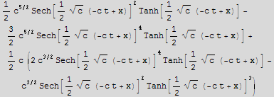
(![]() (x-ct)) is a solution. Compare the operator and the expression representations of the PDE for this purpose.
(x-ct)) is a solution. Compare the operator and the expression representations of the PDE for this purpose.
![candidateSolution = c/2Sech[c^(1/2)/2 (x - c t)]^2 ;](HTMLFiles/index_17.gif)
![]()

![]()
![]()
![]()

![]()
![]()
Notice the slight difference in the PDE in the two forms. In both cases ofcourse the solution is verified correctly. The expression representation is shorter, but using simplify we obtain the same final answer in both cases
3. Here is a complicated expression
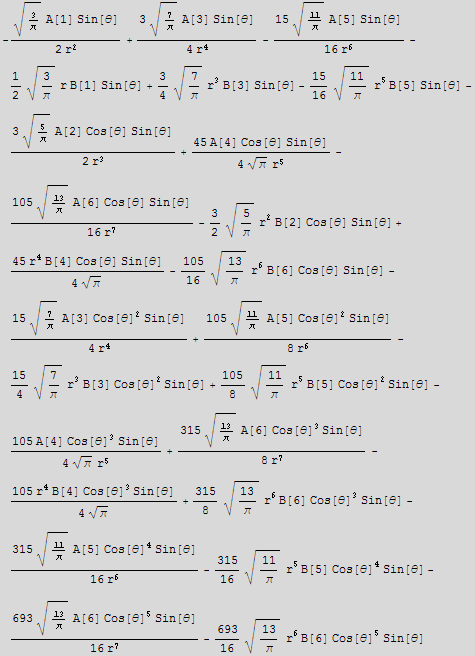
![]()

which is a typical form of a trial solution for many types of problems with spherical symmetry.
a) In one line of code, find all the terms of the series proportional to Cos[θ]^2
![]()

b) in one line of code, construct a list containing the powers of r that occur in the terms you found in part a.
![]()
![]()
4) Here is a differential equation:
![]()
![]()
![]()
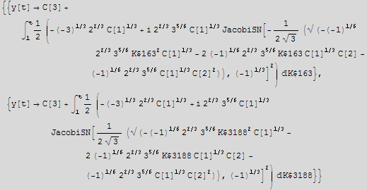
a)Verify that DSolve either cannot solve the equation, or produces a very complicated implicit solution, depending on which version of Mathematica you are running.
![]()
![]()

b) Use a pure function to substitute a trial solution of the form a ![]() .
.
![]()
![]()
c) The result should be a polynomial in t. Think carefully about the conditions for a polynomial of this type to vanish for all t. Find values of a and n which make the solution work for all t and verify that your solution works.
For the polynomial to be zero everywhere, then f(a,n) t^-(3+n) = - g(a,n) t^(-2+2n), which happens when the powers t is raised to are equal, and when f=g. So we solve to find when this happens.

![]()
![]()
![]()
![]()
![]()
![]()
![]()
![]()
![]()
![]()
![]()
We see that n must be -1. When n = -1, this means a = 6.
We also have the solution of a=0 which will work for any n.
Hence final solution is: n=-1 and a=6, and a=0 for any n.
In fact, when a=0 the trial solution will be y=0.It is a special solution which should be ignored.
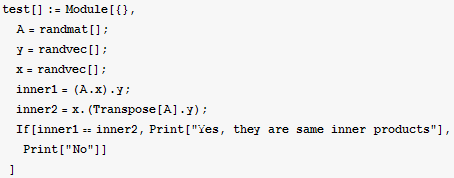
5. Explore properties of matrix Transpose: show that < Ax,y>=<x,![]() y> for a random x, y and A. Make a function randvec[] that makes a random 3-vector, and randmat[] that makes a random 3x3 matrix. Use these to make a function test[] which will compute the 2 inner products and test if they are equal. Verify the relation for a number of cases.
y> for a random x, y and A. Make a function randvec[] that makes a random 3-vector, and randmat[] that makes a random 3x3 matrix. Use these to make a function test[] which will compute the 2 inner products and test if they are equal. Verify the relation for a number of cases.
![]()
![]()
![]()
![]()

![]()
![]()
![]()
![]()
![]()
6. Here are 2 vectors:
![]()
![]()
![]()
![]()
![]()
a) Find a vector perpendicular to these vectors using NullSpace, and verify that they are perpendicular.
![]()
![]()
![]()
![]()
![]()
![]()
![]()
![]()
![]()
![]()
![]()
![]()
![]()
![]()
![]()
![[Graphics:HTMLFiles/index_84.gif]](HTMLFiles/index_84.gif)
The above diagram shows geomertically that the vector p, which is the SOLID BLACK line in the diagram is perpendicular to both v1 and v2 vectors (the lines with the colors BLUE and RED). So the vector p, is perpendicular to the plane spanned by v1 and v2 as the diagram also shows.
b) Use Cross to find a vector perpendicular to v1 and v2, and verify that it is proportional to the one you found in a)
![]()
![]()
![]()
![]()
![If[angleBetweenV3Andp == Pi || angleBetweenV3Andp == 0, Print["Vectors are parallel as expected"], Print["Not verified. Something is wrong"]] ;](HTMLFiles/index_89.gif)
![Print["Angle between v3 and p (from part a) is zero or 180, hence Cross product of v1,v2 is proportional to one found in part(a)"] ;](HTMLFiles/index_90.gif)
![]()
![]()
Here are 2 vectors in 5 dimensional space:
![]()
![]()
![]()
![]()
c) Find a vector perpendicular to w1 and w2 using NullSpace.
![]()
![]()
![]()
![]()
Now generate some scales to stretch the basis vectors with. These scales are what we consider to be the coordinates of the position vector itself. Multiply each basis vector by some integer number (I could also have used Real number, but it is more clear if I use Integer multiplier.
![]()
![]()
![]()
![]()
![]()
To verify, dot multiply 's' with w1 and w2 at a time, the result should be zero in both cases
![]()
![]()
![]()
![]()
7. Here is a matrix

a) What is the rank of A?
![]()
![]()
b) Find a value of rhs so that A.x==rhs is a consistent equation.
![]()
![]()
![]()
![]()
![]()
![]()
![]()
![]()
![]()
c) Using your choice of rhs, find the general solution using LinearSolve and NullSpace.
![]()
![]()
![]()
![]()
![]()
![]()
![]()
Where 't' above is any scalar
8. Here is a table of data in {x,y} pairs:
![]()


a) Fit the data to the form y=a ![]() +b x +c. Do this by requiring that this form be true for every data point. This will produce many equations in the three unknowns a, b, c. Use PseudoInverse to solve this overdetermined set of equations to get the best least squared estimates of a,b,c. Compare the data and the fit on the same plot.
+b x +c. Do this by requiring that this form be true for every data point. This will produce many equations in the three unknowns a, b, c. Use PseudoInverse to solve this overdetermined set of equations to get the best least squared estimates of a,b,c. Compare the data and the fit on the same plot.
![]()
![]()
![]()
![]()
![]()
![]()
![]()
![]()
![]()
![[Graphics:HTMLFiles/index_142.gif]](HTMLFiles/index_142.gif)
b) Now use Fit to find the values of a,b,c. The method you used above is the numerical method that Fit uses. Show that the answers obtained are the same both ways.
![]()
![]()
![]()
We see that the Fit command gives the same answer as part(a)
9. (grads) Residues can be used to compute integrals that would otherwise be difficult or impossible. The same is true of sums. We have previously seen that Mathematica can do sums such as
![]()
![]()
The trick for doing sums of the form ![]() g[n] using complex function theory is to find a contour integral that is reasonably easy to do and whose residues are the values g[1], g[2] .., g[n]. The first step is to find a function that has poles at integer values along the real line. Such a function is π Cot[π z].
g[n] using complex function theory is to find a contour integral that is reasonably easy to do and whose residues are the values g[1], g[2] .., g[n]. The first step is to find a function that has poles at integer values along the real line. Such a function is π Cot[π z].
a) Expand π Cot[π z] in a series centered at z=n, with n an integer for several values of n to convince yourself that the poles are there.
b) Construct a proof (or at least a plausibility argument ) that these are the only poles the function has.
c) Now consider the integral ∮ ![]() dz over a contour consisting of a circle centered at the origin of radius R as R->∞. The value of the integral is zero. Show why this is true by examining the behavior of the real and imaginary parts of π Cot[π z] in polar coordinates for fixed θ and large r. Find an upper bound for the integral and show that the upper bound tends to zero for large r.
dz over a contour consisting of a circle centered at the origin of radius R as R->∞. The value of the integral is zero. Show why this is true by examining the behavior of the real and imaginary parts of π Cot[π z] in polar coordinates for fixed θ and large r. Find an upper bound for the integral and show that the upper bound tends to zero for large r.
d) Finally, use the residue theorem to express the integral (which=0) in terms of the sum of the residues. Construct a table using Table of the residues of ![]() for n=-10,-9...9,10. From the structure of the table, explain why
for n=-10,-9...9,10. From the structure of the table, explain why ![]()
![]() =
=![]() .
.
e) Calculate the sum ![]()
![]() using the above technique. (note that this time there are poles not on the real line) Calculate the appropriate residues, and check your answer using Sum.
using the above technique. (note that this time there are poles not on the real line) Calculate the appropriate residues, and check your answer using Sum.
| Created by Mathematica (January 30, 2007) |