Physics 229& 100 Homework #2
Name: Nasser Abbasi

1. Find all real solutions of  =5 -30 +4.  Provide convincing commentary in a Text cell which explains why you have found all of them.

Since this is not a polynomial equation we need to use FindRoot[], which requires an initial guess. So we do a plot first to see where can give the guess at.

Now looking at the plots above, we can determine the roots.

The above are all the real roots found. I used 2 methods to convince myself of this.

Method 1: First by looking at the plot, we see that there can be no more real roots after x=15 since for larger x the exponential terms dominates and increases much faster than the eq2 function which has only x^5 as the largest term. So they not cross again. This can also be seen by plotting for larger and larger x. So the function must continue to increases, so it can not cross the x-axis again. For larger and larger x in the negative direction, the exponential term (eq1) decays rapidly to zero, while x^5 term become the dominant term and it grows larger and larger. Hence eq1 and eq2 curves can never meet again.

Method 2: expend Exp[x] in Taylor series for very large number of terms. This made the terms eq1-eq2 a polynomial equation. Then use Solve. Then count the number of real roots found. I got 4. This below is an example.

2.  a) Consider the function f(z)= dx. Construct a plot of this function for x in the range (0,5).

b) For what value of w is f(w)=250?  

c) If values of f(w) were required repeatedly in a longer calculation, it would be wasteful to recompute the value of the integral each time. It would be more efficient to make a table (using Table) of values, and then to use Fit to find a smooth representation for the values. Find such a fit ( a polynomial in works reasonably well) and show that the fit is within ±0.5 of the exact value by constructing an error plot .

3. The sensitivity of the roots of a polynomial to  the exact value of its coefficients is illustrated by a famous pathological polynomial. This polynomial has -1,-2,-3...-20  as roots.
a) Construct this polynomial using Product and Expand. Verify that the coefficient of the term is the negative of the sum of the n=20 roots. (use Coefficient and Sum).  Verify that the constant term is the product of the roots. These are general properties of polynomials.

b) Verify that NSolve finds all the roots of the polynomial. Now construct a new polynomial by adding 1.0 * to the coefficient of . Use NSolve to find the roots of the new polynomial. Make a plot of their location in the complex plane by constructing a separate list of the real and imaginary parts, and then combining them into {x,y} pairs using Transpose. Make a plot using ListPlot.

Notice how a very small perturbation in one term coefficient made very large change in solution

4. Consider a uniformly charged disk of radius R. Find the electrostatic potential at a point z on the axis; call it potz (set up the appropriate integral using Integrate). Find a series expansion for potz valid for large z. Do this in two different ways:

a) First, make a substitution z->1/ε; in this new formula, ε->0 is equivalent to z->∞. Find the series expansion in ε about zero, and then substitute ε->1/z.

Note: a differential area on the disk is da=r dθ dr

b) Second, expand potz about the point ∞ (see Series). Confirm that you get the same answer both ways. (the second way is obviously easier).

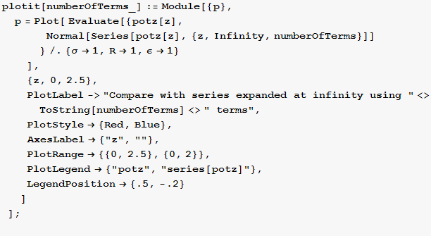
c) If we measure z in units of the disk radius R, we can set R->1; Plot potz and the first two terms of the series expansion on the same graph (set σ and any other constants->1) . Show that the series expansion is a terrible approximation at z=1/2, but is excellent at z=2. The first two terms are called the monopole and the quadrupole terms in the potential. Check your calculation by making sure that the monopole term is the potential of the total charge concentrated at the origin.

We see from the plots above the following: The BLUE curve represents potz expressed in series expansion around infinity, while the RED curve is potz function. We see that for z less than around .5, the approximation is very bad. The approximation improves quickly after about z=1. At z=2 for example, one sees no difference between the series expansion and potz itself.

5.

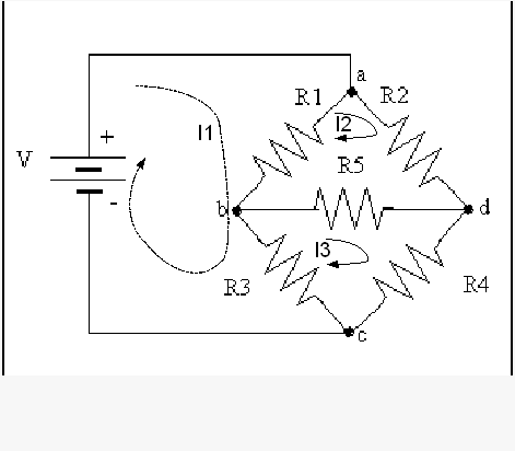
Find an expression for the voltage at point d in the circuit above. Go here for a reminder about rules for circuits. Clearly describe what variables you are using and what principles you use to generate your equations.  A good way to do this is with a drawing.You should cut and paste the drawing above into a graphics package  such as Paint that works with bit map graphics and add current labels and arrows.

The above diagram shows the method to use for generating the equations. We have 3 loops. Using Kirchoff laws, we know that the sum of voltages in each loop must add to zero. Using this we generate 3 equations (one per loop), which we solve for I1,I2,I3. Next we use Ohm's law to find Voltage at point d.

Now we can find the voltage at point d

6. Graphics exercises.
a) Use Mathematica to make a drawing  of unit vectors emanating from the origin that looks like

Use Arrow, which  requires loading a package, as described here.  Arrow is similar to Line; the arguments are Arrow[ {tail},{head}] , where head and tail are vectors that specify the location of the head and tail of the arrow.  Use Table to make a list of Arrows.

b) Make another drawing which adds a small red circle at the end of each arrow . Information about graphics directives to change properties such as color are described here.

c) The equation -= 6 x y defines a curve in the plane. Plot this curve using either ContourPlot or ImplicitPlot as described here.

d) Use ContourPlot3D to make a plot of the unit sphere.

e) Use ParametricPlot3D to make a plot of the unit sphere. The {x,y,z} coordinates of the points on a sphere are described here.

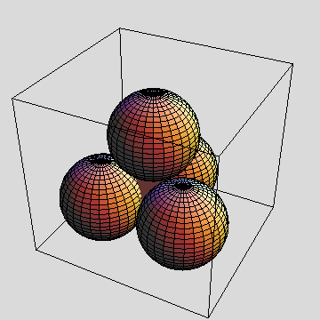
f) Construct a drawing of 4 mutually tangent spheres centered on the vertices of a tetrahedron.  Use ParametricPlot3D to draw the spheres. Turn on RealTime3D so the drawing can be rotated with the mouse.

7. Computational algorithms are said to work in polynomial time if the execution time is proportional to , where N is a characteristic scale of the length of the input data, and n is a fixed constant that characterizes the efficiency of the algorithm. Using the discussion of the computing time for Det as a guide, estimate n for the Mathematica function Eigenvalues. How long would it take to find the eigenvalues of a 3000 x 3000 matrix on your computer? ( Don't actually try to do it).

8 a) Calculate the exact value of the sum 1-+-+...  ( Hint: a convenient way to find an expression for the nth term is to use Fit and a linear function of n  on the terms you know)

write a function that generates the partial sum of the first Nt terms of the series. Make a plot of the value of the partial sums as a function of Nt  from 1 to 50.

How many terms of the sum are required to ensure that the error is less than 0.001 ?

9

Use MonteCarlo integration using Method→MonteCarlo  in NIntegrate to compute the volume of high dimensional spheres.
a) first verify that you get the right answer for a 3 dimensional sphere of radius =1

First I will use spherical coordinates for 3D. Using spherical coordinates, the volume is found by integrating a unit volume. We obtain the formula that V= 8(Sin[φ])drdφdθ

Using the normal Cartesian coordinates systems,we get

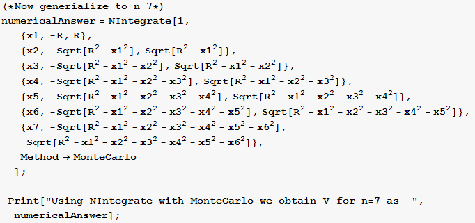
b) Next, calculate the volume of a sphere in 7 dimensions with radius =1

To do this in higher dimensions, I will use the normal Cartesian coordinates systems.

c)( grads)  write a function Vsphere[ndim_] that will use montecarlo integration to calculate the volume of the unit n-sphere in ndim dimensions. Make a table of values and a plot for dnim={2,12}, which shows that  as a function of n, a 5-sphere has the maximum volume and that ( counterintuitively) the volumes of spheres for dimensions >5 decreases rapidly with dimension. You may have to experiment with PrecisionGoal and MaxPoints.
To automatically generate the limits for your function, you will want to make a list of limits called lims, and then use Evaluate[Apply[Sequence,lims]] to splice the arguments into NIntegrate. See Further Examples in the Help for Sequence.

NOTE: I am attempting this as extra, I am not signed as a Grad

Using a formula based on Gamma function for finding sphere Volume in higher n, we can generate the above function.

Created by Mathematica  (January 30, 2007)