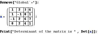
a) Find the determinant of this matrix:
 |
Ok.Next time please keep the marks I made so I know which problem I should look at.
Physics 229& 100 Homework #1
Name: Nasser Abbasi
1. Practice in transcribing expressions into Mathematica syntax
a) Find the determinant of this matrix:

![]()
b) If ![]() , what is
, what is ![]() ?
?

![]()
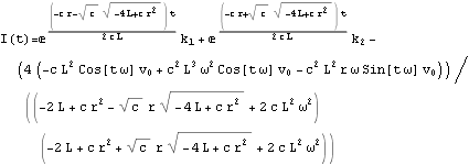
c) In your E&M book, you find the following equation which describes an LCR circuit : ![]() . Use DSolve to find the general solution to the equation.
. Use DSolve to find the general solution to the equation.

d) Find the first 3 terms in the Taylor's series expansion of ![]() about x=0.
about x=0.

![]()
2
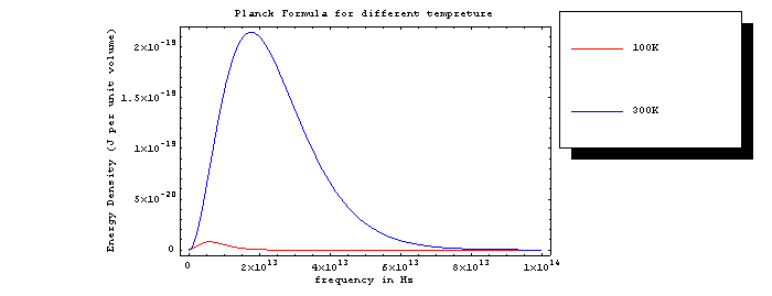
The electromagnetic energy density inside a cavity at temperature T has a distribution of frequencies f. The distribution is given by the famous Planck formula ![]() , where h is Planck's constant, k is Boltzmann's constant, and c is the velocity of light.
, where h is Planck's constant, k is Boltzmann's constant, and c is the velocity of light.
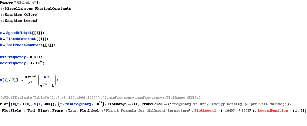
a) Make a plot of the energy density as a function of f for T=100K and 300K. Be sure to include the physically relevant range of f. Make the curves different colors. Make a substitution rule to provide numerical values for the constants.
![]()
b) Find the total energy in the cavity, which is given by the integral of the energy density over frequency. Leave the result in symbolic form( i.e. in terms of h, k, c, etc.) . You might want to include an Assumptions->Re[ ]>0 to avoid If statements in the answer. See examples of this in Integrate.

![]()
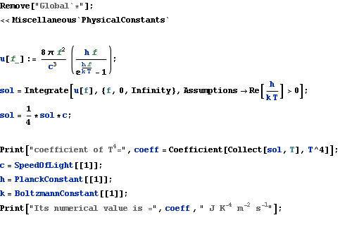
c) The power flux in the radiation is the total energy times the rate at which it moves (which is the speed of light, c) times a geometrical factor (1/4). Evaluate this and find the numerical coefficient of ![]() ; this is the Stefan-Boltzmann constant of radiative transfer.
; this is the Stefan-Boltzmann constant of radiative transfer.
![]()
![]()
3
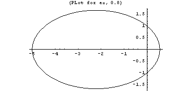
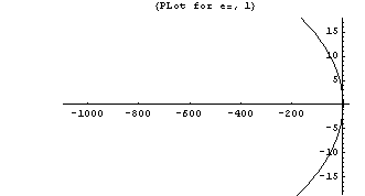
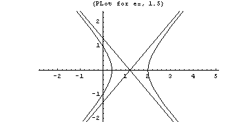
Conic sections can be described by the equation ![]() , where e is the eccentricity, and r and θ are polar coordinates, with x=r Cos[θ] and y=r Sin[θ]. Use ParametricPlot to draw the curves for e=0.8, e=1, and e=1.5
, where e is the eccentricity, and r and θ are polar coordinates, with x=r Cos[θ] and y=r Sin[θ]. Use ParametricPlot to draw the curves for e=0.8, e=1, and e=1.5

4
The temperature in degrees Fahrenheit F is related to the temperature in degrees centigrade C by the formula F=![]() . The temperature in Kelvin K is related to the centigrade temperature by C-273=K. Use Table to make a table which gives all three temperatures for K=0,300 in 10 degree increments. Use TableForm with TableHeadings to make a nice printout.
. The temperature in Kelvin K is related to the centigrade temperature by C-273=K. Use Table to make a table which gives all three temperatures for K=0,300 in 10 degree increments. Use TableForm with TableHeadings to make a nice printout.

| Kelvin | Centigrade | Fahrenheit |
| 0 | -273. | -459.4 |
| 10 | -263. | -441.4 |
| 20 | -253. | -423.4 |
| 30 | -243. | -405.4 |
| 40 | -233. | -387.4 |
| 50 | -223. | -369.4 |
| 60 | -213. | -351.4 |
| 70 | -203. | -333.4 |
| 80 | -193. | -315.4 |
| 90 | -183. | -297.4 |
| 100 | -173. | -279.4 |
| 110 | -163. | -261.4 |
| 120 | -153. | -243.4 |
| 130 | -143. | -225.4 |
| 140 | -133. | -207.4 |
| 150 | -123. | -189.4 |
| 160 | -113. | -171.4 |
| 170 | -103. | -153.4 |
| 180 | -93. | -135.4 |
| 190 | -83. | -117.4 |
| 200 | -73. | -99.4 |
| 210 | -63. | -81.4 |
| 220 | -53. | -63.4 |
| 230 | -43. | -45.4 |
| 240 | -33. | -27.4 |
| 250 | -23. | -9.4 |
| 260 | -13. | 8.6 |
| 270 | -3. | 26.6 |
| 280 | 7. | 44.6 |
| 290 | 17. | 62.6 |
| 300 | 27. | 80.6 |
5
Consider the system of linear equations
| I x | +y | +z | -I w | = | 0 |
| x | +I y | -I z | +w | = | I |
| x | -y | = | 1 | ||
| x | -I y | = | 0 |
a) Solve for x,y,z,w using Solve.
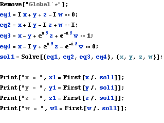
![]()
![]()
![]()
![]()
b) Extract the matrix of coefficients. One convenient way to do this is to use Input-> Create Table/Matrix/Palette->Matrix. Solve for x,y,z,w using Inverse. Convince yourself you get the same answers as in part a.
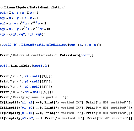

![]()
![]()
![]()
![]()
![]()
![]()
![]()
![]()
![]()
6
The Bernoulli numbers ![]() appear in many formulas you will find in tables of integrals. They are defined as the coefficients of powers of z in the expansion
appear in many formulas you will find in tables of integrals. They are defined as the coefficients of powers of z in the expansion
 =1+
=1+![]() z+
z+![]()
![]() +
+![]()
![]() ...
...
Write a function bern[n] that returns the nth Bernoulli number. Use Series and Coefficient[expr,form] to extract the coefficient. Use the function and the Table command to make a table of the first 20 Bernoulli numbers. Compare with the built-in function BernoulliB.

| n | bern[n] | BernoulliB[n] |
| 1 | ||
| 2 | ||
| 3 | 0 | 0 |
| 4 | ||
| 5 | 0 | 0 |
| 6 | ||
| 7 | 0 | 0 |
| 8 | ||
| 9 | 0 | 0 |
| 10 | ||
| 11 | 0 | 0 |
| 12 | ||
| 13 | 0 | 0 |
| 14 | ||
| 15 | 0 | 0 |
| 16 | ||
| 17 | 0 | 0 |
| 18 | ||
| 19 | 0 | 0 |
| 20 |
7
Consider the quadratic equation ![]() , where R1 and R2 are independent random numbers uniformly distributed on [0,1] .
, where R1 and R2 are independent random numbers uniformly distributed on [0,1] .
a) For each choice of random coefficients R1 and R2, the equation has two solutions, x1 and x2. Write a function printsol[neq_] which prints out x1 and x2 for neq randomly generated equations. Use a Do loop. Execute the function for neq->15.
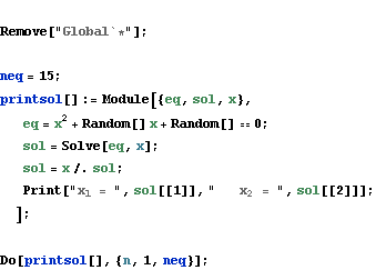
![]()
![]()
![]()
![]()
![]()
![]()
![]()
![]()
![]()
![]()
![]()
![]()
![]()
![]()
![]()

![]()
![]()
![]()
![]()
![]()
![]()
![]()
![]()
![]()
![]()
![]()
![]()
![]()
![]()
![]()
![]()
b) Write a function reimxy[neq_] which computes the solutions x1 and x2 discussed above, and plots the location of each point in the complex plane. Initialize a list xy={}, and use Re, Im, AppendTo, ListPlot, and Do. Execute the function for neq->5000. What fraction of the solutions are Real, i.e. have zero imaginary part? Use a counter and If.

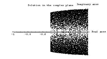
![]()
8
Find the center of mass of a solid half sphere of radius R . Recall that the position of the center of mass is ![]() , where M is the total mass and ρ is the density. Include a diagram which specifies your coordinate system. Go here for a reminder about how to do this.
, where M is the total mass and ρ is the density. Include a diagram which specifies your coordinate system. Go here for a reminder about how to do this.

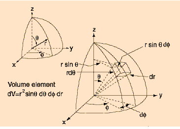

![]()
9 (grads only)
The wavefunctions for the quantum mechanical harmonic oscillator are proportional to ![]()
![]() (x) where
(x) where ![]() (x) are the Hermite polynomials defined by
(x) are the Hermite polynomials defined by ![]() (x)=
(x)=![]()
![]()
![]() . Write a function hermite[n] which returns the nth Hermite polynomial. Compare your answer with the built-in function HermiteH[n,x].Write a function psi[n] that returns the nth harmonic oscillator wave function. Make sure that your wave functions are normalized, ie that
. Write a function hermite[n] which returns the nth Hermite polynomial. Compare your answer with the built-in function HermiteH[n,x].Write a function psi[n] that returns the nth harmonic oscillator wave function. Make sure that your wave functions are normalized, ie that ![]() =1. Plot psi[13] and psi[13]^2, the probability density of finding the particle at x. (See the examples section of Plot for the trick for getting Plot to work properly.)
=1. Plot psi[13] and psi[13]^2, the probability density of finding the particle at x. (See the examples section of Plot for the trick for getting Plot to work properly.)
10 (grads only)
van der Waals attraction to a wall
van der Waals interactions between molecules produce an attractive interaction described by a potential of the form ![]() , where r is the distance between 2 molecules. Show that the interaction energy between a molecule and a half space ( a solid wall) is
, where r is the distance between 2 molecules. Show that the interaction energy between a molecule and a half space ( a solid wall) is ![]() if the molecule is a distance h from a wall with density of molecules ρ.
if the molecule is a distance h from a wall with density of molecules ρ.
The molecule is at vector position x1={0,0,h}
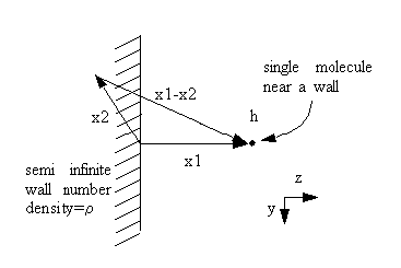
x2={x,y,z} is the position of a typical molecule in the wall, and ranges over the region z<0 . If the number density of molecules in the solid wall is ρ, the potential energy of interaction between the molecule at x1 and all of the molecules in the wall is ∫∫∫ dx dy dz, where the range of integration is over the solid half space.
| Created by Wolfram Mathematica 6.0 for Students - Personal Use Only (24 February 2008) |