HW 5, Problems 5.7
EECS 203A, UCI, Fall 2004

by Nasser Abbasi

Question

TextBook: Digital Image Processing, 2nd edition. By Gonzalez and Woods.

The white bars in the test pattern shown below are 7 pixels wide and 210 pixels high. The separation between bars is 17 pixels. What would this image look like after application of
(a) 3x3 Max filter?
(b) 7x7 ?
(c) 9x9 ?

Answer

Median filter is given by whereis the image data under the filter.

Load the original Image and display it first. I downloaded the image from the text book website, and used InfranView to get the image information to find how many pixels the whole image is, then read in into Mathematica to display it.

In[27]:=

Out[32]=

In the original image,the vertical white bars look like this (displaying the top end of the white bar) we see that the white bar top starts at row number 24,we see that the strip is 7 pixels wide.

3x3 Filter

Now construct each filter, and apply them to the above image

In[33]:=

Out[35]//MatrixForm=

Filter the image with Median 3x3 and display

In[36]:=

Out[37]=

Show the top edge of the white bar BEFORE processing

In[38]:=

Out[38]=

Show the top edge of the white bar AFTER processing

In[39]:=

Out[39]=

Look at the data before:

In[40]:=

Out[40]//MatrixForm=

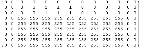
Look at the data after filtering

In[41]:=

Out[41]//MatrixForm=

So we see that the white bar is now is wider, it is 9 pixels wide.  And will be 4 rows longer, it will be 214 pixels high

7x7 Filter

In[42]:=

Now show the top of the white strip. Look now how much more wide it is

In[45]:=

Out[45]=

In[54]:=

Out[54]//MatrixForm=

So we see that the white bar is now is wider, it is 13 pixels wide. and will be 12 rows longer, so 222 pixels high

9x9 Filter

In[55]:=

Out[57]=

In[58]:=

Out[58]=

In[67]:=

Out[67]//MatrixForm=

So we see that the white bar is now is wider, it is 15 pixels wide. and will be 16 rows longer, so 226 pixels high

3D plots

I'll now display the 3 images in 3D to better illustrate the filter result. I will only plot the region near the ends of the top of the first white strips.

In[68]:=

Out[68]=

Out[69]=

Out[70]=

Out[71]=

Created by Mathematica  (November 16, 2004)