HW 5, Problems 5.5
EECS 203A, UCI, Fall 2004

by Nasser Abbasi

Question

TextBook: Digital Image Processing, 2nd edition. By Gonzalez and Woods.

The white bars in the test pattern shown below are 7 pixels wide and 210 pixels high. The separation between bars is 17 pixels. What would this image look like after application of
(a) 3x3 contraharmonic mean filter with Q=-1?
(b) 7x7 ?
(c) 9x9 ?

Answer

CMF is given by whereis the image data under the filter.

Load the original Image and display it first. I downloaded the image from the text book website, and used InfranView to get the image information to find how many pixels the whole image is, then read in into Mathematica to display it.

In[9]:=

Out[14]=

In the original image,the vertical white bars look like this (displaying the top end of the white bar) we see that the white bar top starts at row number 24,we see that the strip is 7 pixels wide.

In[15]:=

Out[15]//MatrixForm=

3x3 Filter

Now construct each ARM filter, and apply them to the above image

In[16]:=

Out[18]//MatrixForm=

Filter the image with HMF3 and display

In[19]:=

Out[22]=

Show the top edge of the white bar BEFORE processing

In[23]:=

Out[23]=

Show the top edge of the white bar AFTER processing

In[24]:=

Out[24]=

After applying the 3x3 filter, the white bar would blur to the
Look at the data before:

In[25]:=

Out[25]//MatrixForm=

Look at the data after filtering

In[26]:=

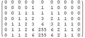
Out[26]//MatrixForm=

So we see that the white bar is now smaller not larger as was the case with Q=1. It is now 5 pixels wide, and  has lost 2 rows at the top and at the bottom by symmetry), hence it will be of 206 pixels high.  So white strips are more narrow.

7x7 Filter

In[27]:=

Out[30]=

Now show the top of the white strip. Look now how much more thin it is

In[32]:=

Out[32]=

In[39]:=

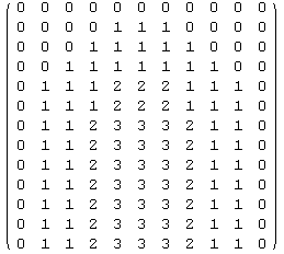
Out[39]//MatrixForm=

We see that now the white bar is  1 pixel wide, and lost 4 rows at the top and 4 rows at the bottom, so it is now 202 pixels high. we see now the white strips are very narrow.

9x9 HMF

In[40]:=

Out[43]=

In[45]:=

Out[45]=

In[57]:=

Out[57]//MatrixForm=

We see that now the white bar has all but disseapered.  

3D plots

I'll now display the 3 images in 3D to better illustrate the filter result. I will only plot the region near the end of the top of the first white strip.

In[58]:=

Out[58]=

Out[59]=

Out[60]=

Out[61]=

Created by Mathematica  (November 16, 2004)