HW4, EECS 203A, Computer Problem (b).
By Nasser Abbasi.
Magnitude of the 2D fourier
transform
3D view of the magnitude of the
fourier transform
Effect of changing ‘c’ scaling
factor
Magnitude of the 2D fourier
transform
3D view of the magnitude of the
fourier transform
Effect of changing ‘c’ scaling
factor
Problem: Generate an image of |F(u,v)| with the DC in the center for the cat and the triangle image.
Conclusion
For the cat image, we see 2 high frequency lines, one vertical through the origin and the second a horizontal line, also through the origin. The vertical line seems to result from the spatial horizontal lines that the carpet texture exhibits. There is also a sharp horizontal like at the top of the image.
The horizontal line in the frequency image seem to result from the spatial line which
is the white to dark edge line to the left of the cat head.
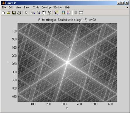
For the triangle image, we see 6 strong lines in the frequency image. 3 of these lines correspond to the 3 edges of the triangle. I am not sure now why I get 6 lines in the frequency image.
Solution
Cat results
Original image
For the cat, this is the original image (480x640) gray level scale, 8 bits per pixel.

Magnitude of the 2D Fourier transform
Below is the Magnitude of the 2D Fourier transform, scaled using s=c log(1+r) for c=22.

3D view of the magnitude of the Fourier transform
This is a 3D view of the magnitude of the Fourier transform.

Effect of changing ‘c’ scaling factor
This below shows the effect of changing the scaling factor ‘c’ in the equation s=c*log(1+r). It shows the |F| plot for different ‘c’ values

Triangle results
Original image

Magnitude of the 2D Fourier transform
Below is the Magnitude of the 2D Fourier transform, scaled using s=c log(1+r) for c=22.
3D view of the magnitude of the Fourier transform
This is a 3D view of the magnitude of the Fourier transform.

Effect of changing ‘c’ scaling factor
This below shows the effect of changing the scaling factor ‘c’ in the equation s=c*log(1+r). It shows the |F| plot for different ‘c’ values

Source code
function nma_EECS_203A_HW4_prob_b
%
% Solve HW4, EECS 203A, computer problem b.
% Determine the 2D fourier transform magnitude
% of an image
%
% by Nasser Abbasi
% EECS 203A, UCI, Fall 2004.
%
M=480; %
rows
N=640; %
columns
fileName='triangle.raw';
fid=fopen(fileName,'r');
f=fread(fid,[N,M],'uint8');
fclose(fid);
f=f';
figure;
imagesc(f,[0 255]);
colormap gray;
colorbar;
title(sprintf('Original raster file %s',fileName));
figure;
F = fft2(f,M,N);
F = fftshift(F); % Center FFT
F = abs(F);
% Takes the magnitude of F
F = round(F);
c=22;
imagesc(c*log(1+F),[0 255]); colormap gray;
title(sprintf('|F| for triangle. Scaled with c
log(1+F), c=%d',c));
xlabel('v'); ylabel('u');
figure;
mesh(1:N,1:M,.6*log(1+F)); colormap jet;
xlabel('v'); ylabel('u');
title(sprintf('3D view of |F| for triangle. Scaled
with c log(1+F), c=%d',c));
figure;
c=1;
for (i=1:25)
subplot(5,5,c);
imagesc(i*log(1+F),[0 255]); colormap gray; title(sprintf('c=%d',c));
c=c+1;
end