![... 2371;, RowBox[{RowBox[{tbl2, =, RowBox[{process, [, RowBox[{1., ,, 1.5}], ]}]}], ;}], }]}]](HTMLFiles/index_1.gif)
HW2, Computer problem, Part (a)
EECS 203A, Digital Image Processing. UCI. Fall 2004
Nasser Abbasi
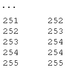
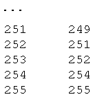
Define the transformation and generate 2 lookup tables and plot the curves. I also list the first and last 5 rows in each table for each curve to better see the values. The first column in the table is the r values and the second column is the s values.
In[27]:=
![... 2371;, RowBox[{RowBox[{tbl2, =, RowBox[{process, [, RowBox[{1., ,, 1.5}], ]}]}], ;}], }]}]](HTMLFiles/index_1.gif)
| 0 | 0 |
| 1 | 6 |
| 2 | 10 |
| 3 | 13 |
| 4 | 16 |

![[Graphics:HTMLFiles/index_3.gif]](HTMLFiles/index_3.gif)
![]()
| 0 | 0 |
| 1 | 0 |
| 2 | 0 |
| 3 | 0 |
| 4 | 1 |

![[Graphics:HTMLFiles/index_6.gif]](HTMLFiles/index_6.gif)
Now set current directory to where the image is (same folder as this note book) and read the image file
In[34]:=
![SetDirectory[ToFileName[Extract["FileName"/.NotebookInformation[EvaluationNotebook[] ... ; rows = 480 ; cols = 640 ; data = FastBinaryFiles`ReadListBinary[fileName, Byte] ;](HTMLFiles/index_7.gif)
Now that the image is read into data, we display it before appying GLT on it.
In[39]:=
![ListDensityPlot[Reverse[Partition[data, cols]], MeshFalse, FrameFalse, ImageSize {rows, cols}, PlotRangeAll, AspectRatioAutomatic] ;](HTMLFiles/index_8.gif)
![[Graphics:HTMLFiles/index_9.gif]](HTMLFiles/index_9.gif)
Now apply first GLT to this image.c=1.0,γ=0.67 and display the result
In[40]:=
![out = applyGLT[Flatten[data], tbl1] ; fileName = "cat_low_gamma.raw" ... [fileName] ; FastBinaryFiles`WriteBinary[strm, Flatten[out], Byte] ; Close[strm] ;](HTMLFiles/index_10.gif)
![[Graphics:HTMLFiles/index_11.gif]](HTMLFiles/index_11.gif)
![]()
Now apply second GLT to this image.c=1.0,γ=1.5 and display the result
In[45]:=
![out = applyGLT[Flatten[data], tbl2] ; fileName = "cat_high_gamma.raw" ; strm = FastB ... OpenWriteBinary[fileName] ; FastBinaryFiles`WriteBinary[strm, Flatten[out], Byte] ; Close[strm] ;](HTMLFiles/index_13.gif)
![[Graphics:HTMLFiles/index_14.gif]](HTMLFiles/index_14.gif)
![]()
Conclusion
With γ=1.5,the new image is darker than the original image.With γ=0.67,the new image is lighter than the original image.Looking at the curves we see that with smaller γ darker areas are spread more over to the lighter gray level,and the reverse happens with higher γ
![]()
![]()
Created by Mathematica (October 19, 2004)