
problem:
solution:
Let \(\left [ \Theta \right ] \) be the dimension of temperature.
A small note on how to scale the dependent variable and the independent variable in the problem.
For the dependent variable, say \(y\left ( t\right ) \), if the problem does not say which problem parameters to scale against, then look for a parameter or a combination of these parameters with the appropriate dimension of that of the dependent variable such the parameter is the largest value. This way we are measuring the depndent variable relative to the largest parameter in the problem. Hence when we write \(\tilde {y}=\frac {y}{s}\) where \(s\) is the largest parameter in the problem with dimension of \(y.\)
For the indepenent variable (typically this will be time), we look for the larget rate of change in the problem involving this variable, and scale the time relative to this rate. Hence we write \(\tilde {t}=\frac {t}{s}\) where now \(s\) is the smallest parameter in the problem with dimension of \(t\).
Now we start with the solution of the problem.
(a) \(\frac {dT}{dt}=q\times \)number\(,\) hence
i.e. the dimension of \(q\) is temperature over time.
Now to find the dimension of \(k.\) since\(\frac {dT}{dt}=k\left ( T-T_{f}\right ) \), then \(\left [ \frac {\Theta }{T}\right ] =\left [ k\right ] \left [ \Theta \right ] \,\ \) hence
Now to find the dimension of \(A\). Since \(e^{-\frac {A}{T}}\) must be a numerical dimensionless value, then \(A\) must have the same dimensions as \(T\) (which has dimension \(\left [ \Theta \right ] \)), hence
(b) The constants in this problem are \(T_{f},T_{0},q,k,A\), and the dependent variable is \(T\) which is the temperature of the sample, and the independent variable is \(t\) which is time.
Hence to reduce the above ODE to dimensionless form, we need to transform the dependent and the independent variables to dimensionless variables. Start with the dependent variable \(T\).
We write \(\tilde {T}=\frac {T}{s}\), so we need to find \(s\) as a combination using the constants \(T_{f},T_{0},q,k,A\) in the ODE which would have the dimension of temperature to make \(\tilde {T}\) dimensionless.
This is easy, since we are told to use \(T_{f}\), hence \(s=T_{f}\) and so
Now we need to transform the independent variable, which is time \(t\), hence we write \(\tilde {t}=\frac {t}{s}\), and we need to find \(s\) as a combination of the constants \(T_{f},T_{0},q,k,A\) which has a dimension of time.
Looking above at the dimensions of these constants, we see that the following combinations are possible: \(\left \{ \frac {1}{k},\frac {A}{q},\frac {T_{f}}{q},\frac {T_{0}}{q}\right \} .\) Now since we want the new time scale to be large when the heat loss is large, and since the heat loss is proportional to \(k\), hence we pick \(s=\frac {1}{k}\), this will make \(s\) small and \(\frac {t}{s}\) will then be large. Therefor
Now we convert the ODE to non dimensional using (1) and (2)
but from (2) we have \(\frac {d\tilde {t}}{dt}=k\), hence
and since \(T=T_{f}\tilde {T}\), then the above becomes
Hence the ODE \(\frac {dT}{dt}=qe^{\frac {-A}{T}}-k\left ( T-T_{f}\right ) \) becomes (after replacing \(T\) by \(T_{f}\tilde {T}\) in the RHS)
Now \(\frac {q}{T_{f}k}\) must be dimensionless. Verify \(\frac {\left [ \frac {\Theta }{T}\right ] }{\left [ \Theta \right ] \left [ \frac {1}{T}\right ] }=1\) . OK, so the above ODE can be written as
where \(\beta =\frac {q}{T_{f}k}\)
Note \(e^{\frac {-A}{T_{f}\tilde {T}}}\) must be dimensionless also, since \(\frac {-A}{T_{f}\tilde {T}}\) is dimensionless.
For the initial conditions, now it becomes \(\tilde {T}_{o}=\frac {T}{T_{f}}\)
problem:
solution:
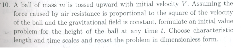
First draw a free body diagram. Assume the ball is moving upwards, and assume the drag force is given by \(F_{d}=k\left ( y^{\prime }(t)\right ) ^{2}\ \)where \(k\) is constant of proportionality, and weight of ball is given by \(W=mg\ \)
Now to obtain the equation of motion, apply Newtons second law \(F=ma\), hence we obtain
Notice that we assumed the positive \(y\) direction is upwards. Hence we obtain the equation of motion
with the initial conditions
This problem has the following constants: \(\left \{ V,m,g,k,y_{0}\right \} \). To find the dimensions of \(k\), since \(k\left ( \frac {dy\left ( t\right ) }{dt}\right ) ^{2}\) must have the dimension of Newton \(\left [ N\right ] \) then we write
\(\left [ N\right ] =\left [ k\left ( \frac {dy\left ( t\right ) }{dt}\right ) ^{2}\right ] \rightarrow \left [ M\frac {L}{T^{2}}\right ] =\left [ k\right ] \left [ \frac {L}{T}\right ] ^{2}\)
and \(\left [ g\right ] =\left [ \frac {L}{T^{2}}\right ] \), and \(\left [ m\right ] =\left [ M\right ] \), and \(\left [ V\right ] =\left [ \frac {L}{T}\right ] \), and \(y_{0}=\left [ L\right ] \), hence we write
Now we can start scaling the ODE.
The dependent variable is \(y\left ( t\right ) \), and the independent variable is \(t\). Hence we write \(\tilde {y}=\frac {y}{s}\), where \(\left [ s\right ] =\left [ L\right ] \), so using the above constants, we need to find a combination which has the dimension of length \(\left [ L\right ] \). Clearly \(y_{0}\) is one possibility. There are other combinations which give the dimension of length. We find the following: \(\left \{ y_{0},\frac {m}{k},\frac {V^{2}}{g}\right \} \).
Now we get to the hard part of these scaling problems. Which combination to choose? The problem did not give us a hint on this. I choose \(s=\frac {V^{2}}{g}\), therefor
Now for the time scale. We write \(\tilde {t}=\frac {t}{s}\) where \([s]=\left [ T\right ] \), looking at the above constants, we need a combination with dimension \(\left [ T\right ] \), we see that \(s=\frac {V}{g}\) has the dimension of time, so we have
Now that we have the scaling completed, we apply them to scale the ODE. In otherwords, we need to rewrite the ODE so that instead of using\(\left \{ y,t\right \} \) it will use \(\left \{ \tilde {y},\tilde {t}\right \} \)
\(\frac {dy}{dt}=\frac {dy}{d\tilde {t}}\frac {d\tilde {t}}{dt}\), but \(\frac {d\tilde {t}}{dt}=\frac {g}{V}\), hence
and \(\frac {d^{2}y}{dt^{2}}=\frac {d}{dt}\left ( \frac {dy}{dt}\right ) =\frac {d}{d\tilde {t}}\left ( \frac {dy}{dt}\right ) \frac {d\tilde {t}}{dt}=\frac {d}{d\tilde {t}}\left ( \frac {g}{V}\frac {dy}{d\tilde {t}}\right ) \frac {g}{V}\) hence
Hence the scaled ODE is
Now replace \(y\rightarrow \frac {V^{2}}{g}\tilde {y}\)
Lets us now verify the above is dimensionless. Looking at \(\left [ \frac {k}{m}\frac {V^{2}}{g}\right ] \rightarrow \left [ \frac {M}{L}\right ] \left [ \frac {1}{M}\right ] \left [ \frac {L}{T}\right ] ^{2}\left [ \frac {1}{\frac {L}{T^{2}}}\right ] \rightarrow \left [ \frac {M}{L}\right ] \left [ \frac {1}{M}\right ] \left [ \frac {L^{2}}{T^{2}}\right ] \left [ \frac {T^{2}}{L}\right ] \)
Hence \(\left [ \frac {k}{m}\frac {V^{2}}{g}\right ] \rightarrow 1\) (like magic)
So the dimensionless ODE is
where \(\beta =\frac {k}{m}\frac {V^{2}}{g}\)
Now for the initial conditions in terms of the new scaled variables. Since
hence
and \(V=\frac {dy\left ( 0\right ) }{dt}=\frac {dy\left ( 0\right ) }{d\tilde {t}}\frac {d\tilde {t}}{dt}=\frac {V^{2}}{g}\frac {d\tilde {y}\left ( 0\right ) }{d\tilde {t}}\frac {d\tilde {t}}{dt}\), but \(\frac {d\tilde {t}}{dt}=\frac {g}{V}\) hence
\(\frac {dy\left ( 0\right ) }{dt}=\frac {V^{2}}{g}\frac {d\tilde {y}\left ( 0\right ) }{d\tilde {t}}\frac {g}{V}\rightarrow V\frac {d\tilde {y}\left ( 0\right ) }{d\tilde {t}}\)
So \(\frac {d\tilde {y}\left ( 0\right ) }{d\tilde {t}}=\frac {1}{V}\frac {dy\left ( 0\right ) }{dt}\), but \(\frac {dy\left ( 0\right ) }{dt}=V\), therefor
So the equation of motion in scaled dimensionless form is
with initial conditions
and