HW 14 Mathematics 503, Mathematical Modeling, CSUF , August 6, 2007

Nasser M. Abbasi

October 8, 2025

1 Problem 9 page 346 section 6.2 (PDE’s)

Find all solutions to the heat equation $u_{t}=\kappa u_{xx}$ of the form $u\left ( x,t\right ) =U\left ( z\right ) $ where $z=\frac {x}{\sqrt {\kappa t}}$

We have that $z\left ( x,t\right ) =\frac {x}{\sqrt {\kappa t}}$, hence $\frac {\partial z}{\partial x}=\frac {1}{\sqrt {\kappa t}}$ and $\frac {\partial ^{2}z}{\partial x^{2}}=0$ and $\frac {\partial z}{\partial t}=-\frac {x}{2}\left ( \kappa t\right ) ^{-\frac {3}{2}}\kappa =\frac {-x}{2}\frac {t^{-\frac {3}{2}}}{\sqrt {k}}$

\begin{align*} u_{x}\left ( x,t\right ) & =U^{\prime }\left ( z\right ) \frac {\partial z}{\partial x}\\ & =U^{\prime }\left ( z\right ) \frac {1}{\sqrt {\kappa t}}\end{align*}

\begin{align*} u_{xx}\left ( x,t\right ) & =U^{^{\prime \prime }}\left ( z\right ) \frac {1}{\sqrt {\kappa t}}\frac {\partial z}{\partial x}\\ & =U^{^{\prime \prime }}\left ( z\right ) \frac {1}{\kappa t}\end{align*}

\begin{align*} u_{t}\left ( x,t\right ) & =U^{\prime }\left ( z\right ) \frac {\partial z}{\partial t}\\ & =\frac {-x}{2}U^{\prime }\left ( z\right ) \frac {t^{-\frac {3}{2}}}{\sqrt {k}}\end{align*}

\begin{align*} u_{t} & =\kappa u_{xx}\\ \frac {-x}{2}U^{\prime }\left ( z\right ) \frac {t^{-\frac {3}{2}}}{\sqrt {k}} & =\kappa U^{^{\prime \prime }}\left ( z\right ) \frac {1}{\kappa t}\\ \frac {-x}{2\sqrt {kt}}U^{\prime }\left ( z\right ) & =U^{^{\prime \prime }}\left ( z\right ) \end{align*}

\[ \fbox {$U^{^{\prime \prime }}\left ( z\right ) +\frac {1}{2}z\ U^{\prime }\left ( z\right ) =0$}\]

Let $U^{^{\prime }}\left ( z\right ) =y\left ( z\right ) ,$ hence the above becomes

\begin{align*} y^{\prime }+\frac {1}{2}z\ y & =0\\ \frac {y^{\prime }}{y} & =-\frac {1}{2}z\\ \frac {1}{y}\frac {dy}{dz} & =-\frac {1}{2}z\\ \frac {1}{y}dy & =-\frac {1}{2}zdz \end{align*}

\begin{align*} U\left ( z\right ) & =\int y\left ( z\right ) dz+B\\ & =A\int e^{\frac {-1}{4}z^{2}}dz+B \end{align*}

I think now I need to write the above in terms of $x,t$ again. Fix time, and change $x$ and so we have $dz=\frac {\partial z}{\partial x}dx=\frac {1}{\sqrt {\kappa t}}dx$ and the above integral becomes

\[ u\left ( x,t;\xi \right ) =\int A\left ( \xi \right ) e^{\frac {-\left ( x-\xi \right ) ^{2}}{4\kappa t}}\frac {1}{\sqrt {\kappa t}}d\xi +B\left ( \xi \right ) \]

for any $\xi $ location along the space dimension $x$, where $A\left ( \xi \right ) ,B\left ( \xi \right ) $ are functions that depend on the value $\xi $

2 Problem 3 page 365 section 6.2 (PDE’s)

\begin{align*} u_{t} & =\nabla ^{2}u\ \ \ \ \ \ \ \ \ \ \ \ \ \ \ \mathbf {x}\in \Omega ,t>0\\ u\left ( \mathbf {x},0\right ) & =f\left ( \mathbf {x}\right ) \ \ \ \ \ \ \ \ \ \ \ \ \ \ \mathbf {x}\in \Omega \\ u\left ( \mathbf {x},t\right ) & =g\left ( \mathbf {x}\right ) \ \ \ \ \ \ \ \ \ \ \ \ \ \mathbf {x}\in \partial \Omega ,t>0 \end{align*}

First note that $\nabla ^{2}u\equiv \frac {\partial ^{2}u}{\partial x_{1}^{2}}+\frac {\partial ^{2}u}{\partial x_{2}^{2}}+\cdots +\frac {\partial ^{2}u}{\partial x_{n}^{2}}$ i.e. the Laplacian.

Proof by contradiction. Assume there is no unique solution. Let $u_{1}\left ( x,t\right ) $ and $u_{2}\left ( x,t\right ) $ be 2 diﬀerent solutions to the above PDE. Let $w\left ( x,t\right ) $ be the diﬀerence between these 2 solutions. i.e. $w\left ( x,t\right ) =u_{1}\left ( x,t\right ) -u_{2}\left ( x,t\right ) $, hence $w\left ( x,t\right ) $ must satisfy the following conditions: it must be zero at the boundaries $\mathbf {x}\in \partial \Omega $ for all time, and also it must be zero inside $\Omega $ initially. Hence

\begin{align*} w\left ( \mathbf {x},0\right ) & =0\ \ \ \ \ \ \ \ \ \ \ \ \ \mathbf {x}\in \Omega \\ w\left ( \mathbf {x},t\right ) & =0\ \ \ \ \ \ \ \ \ \ \ \ \ \mathbf {x}\in \partial \Omega ,t>0 \end{align*}

Now if we can show that $w\left ( \mathbf {x},t\right ) =0$ for $t>0$ inside $\Omega $, then this would imply that $u_{1}\left ( x,t\right ) =u_{2}\left ( x,t\right ) $, showing a contradiction, hence completing the proof.

i.e. we need to show that $w_{t}\left ( \mathbf {x},t\right ) =\nabla ^{2}w\left ( \mathbf {x},t\right ) $ yields a solution $w\left ( \mathbf {x},t\right ) =0$ for $\mathbf {x}\in \Omega ,t>0$

First we note that $E\left ( 0\right ) =0\,$since $w\left ( \mathbf {x},0\right ) =0$ from the initial conditions above.

\begin{align*} E^{\prime }\left ( t\right ) & =\frac {\partial }{\partial t}\int _{\Omega }w^{2}\left ( \mathbf {x},t\right ) d\mathbf {x}\\ & =\int _{\Omega }\frac {\partial }{\partial t}w^{2}\left ( \mathbf {x},t\right ) d\mathbf {x}\\ & =\int _{\Omega }2w\left ( \mathbf {x},t\right ) \ \frac {\partial }{\partial t}w\left ( \mathbf {x},t\right ) \ d\mathbf {x}\end{align*}

But $\frac {\partial }{\partial t}w\left ( \mathbf {x},t\right ) =\nabla ^{2}w\left ( \mathbf {x},t\right ) $ from the PDE itself, hence the above becomes

\begin{equation} E^{\prime }\left ( t\right ) =2\int _{\Omega }w\left ( \mathbf {x},t\right ) \ \nabla ^{2}w\left ( \mathbf {x},t\right ) \ d\mathbf {x} \tag {1}\end{equation}

\[ \int _{\Omega }\left ( u\nabla ^{2}w+\nabla u\cdot \nabla w\right ) d\mathbf {x}=\int _{\partial \Omega }u\frac {dw}{dn}dA \]

\begin{align} \int _{\Omega }\left ( w\nabla ^{2}w+\nabla w\cdot \nabla w\right ) d\mathbf {x} & =\int _{\partial \Omega }w\frac {dw}{dn}dA\nonumber \\ \int _{\Omega }w\nabla ^{2}w\ d\mathbf {x}+\int _{\Omega }\nabla w\cdot \nabla w\ d\mathbf {x} & =\int _{\partial \Omega }w\frac {dw}{dn}dA\nonumber \\ \int _{\Omega }w\nabla ^{2}w\ d\mathbf {x} & =\int _{\partial \Omega }w\frac {dw}{dn}dA-\int _{\Omega }\nabla w\cdot \nabla w\ d\mathbf {x} \tag {2}\end{align}

Comparing (1) and (2) we see that LHS of (2) is $\frac {1}{2}E^{\prime }\left ( t\right ) $ Hence the above become

\[ \frac {1}{2}E^{\prime }\left ( t\right ) =\int _{\partial \Omega }w\frac {dw}{dn}dA-\int _{\Omega }\nabla w\cdot \nabla w\ d\mathbf {x}\]

But $\nabla w\cdot \nabla w=\left \Vert \nabla w\right \Vert ^{2}$, so the above becomes

\[ \frac {1}{2}E^{\prime }\left ( t\right ) =\int _{\partial \Omega }w\frac {dw}{dn}dA-\int _{\Omega }\left \Vert \nabla w\right \Vert ^{2}\ d\mathbf {x}\]

But $w\left ( \mathbf {x},t\right ) =0$ on $\partial \Omega $ for $t>0$, since this is the boundary conditions. Hence the above becomes

\[ E^{\prime }\left ( t\right ) =-2\int _{\Omega }\left \Vert \nabla w\right \Vert ^{2}\ d\mathbf {x}\]

Therefore we showed that $E^{\prime }\left ( t\right ) $ is $\leq 0$ since $\int _{\Omega }\left \Vert \nabla w\right \Vert ^{2}\ d\mathbf {x\geq 0}$

So energy inside $\Omega $ is nonincreasing with time. But since $E\left ( 0\right ) =0$ then $E\left ( t\right ) =0$ (since energy can not be negative, this is the only choice left).

Therefore, from $E\left ( t\right ) =\int _{\Omega }w^{2}\left ( \mathbf {x},t\right ) d\mathbf {x}$, we conclude that $w\left ( \mathbf {x},t\right ) =0$ everywhere in $\Omega $ for $t>0$ since $w\left ( \mathbf {x},t\right ) $ is continuous in both its arguments.

Hence we conclude since $w\left ( \mathbf {x},t\right ) =u_{1}\left ( \mathbf {x},t\right ) -u_{2}\left ( \mathbf {x},t\right ) =0$ then $u_{1}\left ( \mathbf {x},t\right ) =u_{2}\left ( \mathbf {x},t\right ) $, then the PDE solution is unique.

3 Problem 5 page 365 section 6.2 Conservation laws

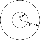
In absence of sources derive the diﬀusion equation for radial motion in the plane $u_{t}=\frac {D}{r}\left ( ru_{r}\right ) _{r}$ from ﬁrst principles. That is, take an arbitrary domain between circles $r=a,r=b$ and apply conservation law for the density $u=u\left ( r,t\right ) $ assuming the ﬂux is $J\left ( r,t\right ) =-Du_{r}$. Assume no sources.

First note that the density $u\left ( r,t\right ) $ is measured in quantity per unit volume.

Consider a cross sectional area through circle $r_{a}=a$. This area is $2\pi hr_{a}$ where $h$ is the width of the strip.

Let $J\left ( r,t\right ) $ be the ﬂux at $r$ at time $t$ , measured in quantity per unit area per unit time.

Hence amount $u$ that passes though cross sectional area at $r_{a}$ , per unit time, is $A\left ( r_{a}\right ) J\left ( r_{a},t\right ) $ where $A\left ( r_{a}\right ) =2\pi hr_{a}$

Similarly, amount $u$ that passes though cross sectional area at $r_{b}$ , per unit time, is $A\left ( r_{b}\right ) J\left ( r_{a},t\right ) $ where $A\left ( r_{b}\right ) =2\pi hr_{b}$

Hence the net amount that ﬂows, per unit time, between $r_{b}$ and $r_{a}$ is $A\left ( r_{a}\right ) J\left ( r_{a},t\right ) -A\left ( r_{b}\right ) J\left ( r_{b},t\right ) $

Since there is no source nor sink inside this region, then the above equal the rate at which the amount $u$ itself changes between $r_{b}$ and $r_{a}$, which is $\frac {d}{dt}\left ( u\left ( r,t\right ) \times \text {volume between }r_{a}\ \text {and }r_{b}\right ) $.

\begin{align*} \frac {d}{dt}\int _{a}^{b}u\left ( r,t\right ) A\left ( r\right ) dr & =A\left ( r_{a}\right ) J\left ( r_{a},t\right ) -A\left ( r_{b}\right ) J\left ( r_{b},t\right ) \\ \int _{a}^{b}u_{t}\left ( r,t\right ) A\left ( r\right ) dr & =A\left ( r_{a}\right ) J\left ( r_{a},t\right ) -A\left ( r_{b}\right ) J\left ( r_{b},t\right ) \end{align*}

Apply fundamental theorem of calculus on the RHS above where $J\left ( a,t\right ) -J\left ( b,t\right ) =\int _{b}^{a}J_{r}dr$ hence the above becomes

\[ \int _{a}^{b}u_{t}\left ( r,t\right ) A\left ( r\right ) dr=\int _{b}^{a}\frac {\partial }{\partial r}\left [ A\left ( r\right ) J\left ( r,t\right ) \right ] dr \]

\[ \int _{a}^{b}u_{t}\left ( r,t\right ) rdr=\int _{b}^{a}\frac {\partial }{\partial r}\left [ rJ\left ( r,t\right ) \right ] dr \]

Changing the limits on the integral in the RHS above to make it match the LHS, we obtain

\[ \int _{a}^{b}u_{t}\left ( r,t\right ) rdr=-\int _{a}^{b}\frac {\partial }{\partial r}\left [ rJ\left ( r,t\right ) \right ] dr \]

Because the above holds for all intervals of integration and the functions involved are continuous, then we can remove the integrals and just write

\[ u_{t}\left ( r,t\right ) r=-\frac {\partial }{\partial r}\left [ rJ\left ( r,t\right ) \right ] \]

Now assuming diﬀusion model for the ﬂux, i.e. $J\left ( r,t\right ) =-Du_{r}\left ( r,t\right ) $, then the above becomes

\[ u_{t}\left ( r,t\right ) r=D\frac {\partial }{\partial r}\left [ ru_{r}\left ( r,t\right ) \right ] \]