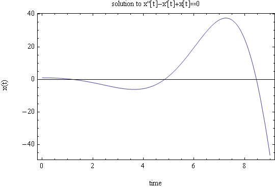
Solve \(\ddot{x}-\dot{x}+x=0\) with \(x_{0}=1\) and \(v_{0}=0\) for \(x\left ( t\right ) \) and sketch the solution
Answer\[ x=x_{h}+x_{p}\] Since there is no forcing function, \(x_{p}\) do not exist, hence \(x=x_{h}\). To determine \(x_{h}\) we first find the characteristic equation and find its root. The characteristic equation is \(\lambda ^{2}-\lambda +1=0\) which has solutions \begin{align*} \lambda _{1} & =\frac{1}{2}+j\frac{\sqrt{3}}{2}\\ \lambda _{2} & =\frac{1}{2}-j\frac{\sqrt{3}}{2} \end{align*}
This is of the form \(\lambda =\alpha \pm \beta j\) (complex conjugates) which has the solution \[ x\left ( t\right ) =e^{\alpha t}\left ( A\cos \beta t+B\sin \beta t\right ) \] Hence \[ \fbox{$x\left ( t\right ) =e^{\frac{1}{2}t}\left ( A\cos \frac{\sqrt{3}}{2}t+B\sin \frac{\sqrt{3}}{2}t\right ) $}\] To find \(A\) and \(B\) we use the initial conditions. At \(t=0\), \(x\left ( 0\right ) =1\), hence\[ \fbox{$A=1$}\] Now \[ \dot{x}\left ( t\right ) =\frac{1}{2}e^{\frac{1}{2}t}\left ( A\cos \frac{\sqrt{3}}{2}t+B\sin \frac{\sqrt{3}}{2}t\right ) +e^{\frac{1}{2}t}\left ( -A\frac{\sqrt{3}}{2}\sin \frac{\sqrt{3}}{2}t+B\frac{\sqrt{3}}{2}\cos \frac{\sqrt{3}}{2}t\right ) \] At \(t=0\), \(v_{0}=0\), hence the above becomes\[ 0=\frac{1}{2}A+B\frac{\sqrt{3}}{2}\] But \(A=1\), hence \[ \fbox{$B=-\frac{1}{\sqrt{3}}$}\] Then the solution is\[ \fbox{$x\left ( t\right ) =e^{\frac{1}{2}t}\left ( \cos \frac{\sqrt{3}}{2}t-\frac{1}{\sqrt{3}}\sin \frac{\sqrt{3}}{2}t\right ) $}\] The solution will blow up in oscillatory fashion due to the exponential term at the front. This is a plot for up to \(t=10\)
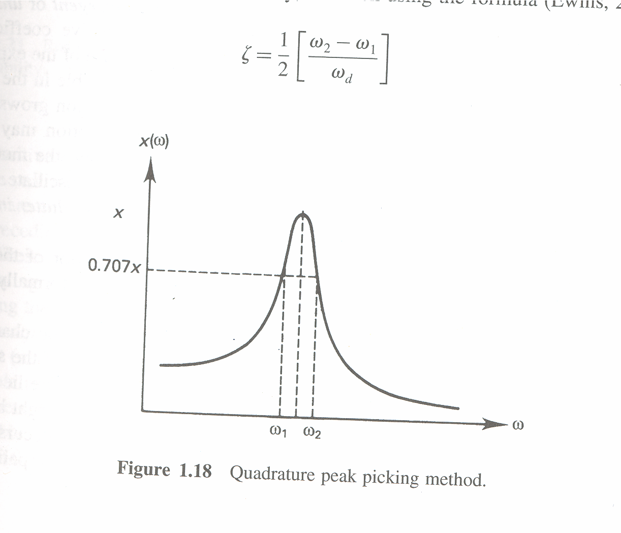
Calculate the maximum value of the peak response (magnification factor) for the system in figure 1.18 with \(\zeta =\frac{1}{\sqrt{2}}\)
Solution
In this figure, the y-axis is the magnitude of the frequency response of the second order system. Hence we must first calculate the frequency response of the system\[ m\ddot{x}+c\dot{x}+kx=u\left ( t\right ) \] or\[ \ddot{x}+2\xi \omega _{n}\dot{x}+\omega _{n}^{2}x=\frac{u\left ( t\right ) }{m}\] Take Laplace transform\begin{align*} s^{2}X\left ( s\right ) +2\xi \omega _{n}sX\left ( s\right ) +\omega _{n}^{2}X\left ( s\right ) & =\frac{1}{m}U\left ( s\right ) \\ X\left ( s\right ) \left ( s^{2}+2\xi \omega _{n}s+\omega _{n}^{2}\right ) & =\frac{1}{m}U\left ( s\right ) \end{align*}
Hence the transfer function is\[ Z\left ( s\right ) =\frac{X\left ( s\right ) }{U\left ( s\right ) }=\frac{1}{m}\frac{1}{s^{2}+2\xi \omega _{n}s+\omega _{n}^{2}}\] Let \(s=j\omega \), the above becomes the frequency response\begin{align*} Z\left ( j\omega \right ) & =\frac{1}{m}\left ( \frac{1}{-\omega ^{2}+2j\xi \omega _{n}\omega +\omega _{n}^{2}}\right ) \\ & =\frac{1}{m\omega _{n}^{2}\left ( 1-\frac{\omega ^{2}}{\omega _{n}^{2}}+2j\xi \frac{\omega }{\omega _{n}}\right ) } \end{align*}
But \(\omega _{n}^{2}=\frac{k}{m}\), hence\[ Z\left ( j\omega \right ) =\frac{1/k}{1-\frac{\omega ^{2}}{\omega _{n}^{2}}+2j\xi \frac{\omega }{\omega _{n}}}\]
Introduce \(G\left ( j\omega \right ) \equiv kZ\left ( j\omega \right ) \) and let \(r=\frac{\omega }{\omega _{n}}\) \[ \fbox{$G\left ( j\omega \right ) =\frac{1}{1-r^{2}+2j\xi r}$}\] Now we can determine the magnitude of the frequency response \begin{align*} \left \vert G\left ( j\omega \right ) \right \vert & =\sqrt{G\left ( j\omega \right ) G^{\ast }\left ( j\omega \right ) }\\ & =\left [ \left ( \frac{1}{1-r^{2}+2j\xi r}\right ) \left ( \frac{1}{1-r^{2}-2j\xi r}\right ) \right ] ^{\frac{1}{2}}\\ & =\frac{1}{\sqrt{\left ( 1-r^{2}\right ) ^{2}+\left ( 2\xi r\right ) ^{2}}} \end{align*}
The maximum of \(\left \vert G\left ( j\omega \right ) \right \vert \) occurs when \(\frac{d\left \vert G\left ( j\omega \right ) \right \vert }{d\omega }=0\) But \[ \frac{d\left \vert G\left ( j\omega \right ) \right \vert }{d\omega }=-\frac{1}{2}\frac{2\left ( 1-r^{2}\right ) \left ( -2r\right ) +4\xi ^{2}\left ( 2r\right ) }{\left [ \left ( 1-r^{2}\right ) ^{2}+\left ( 2\xi r\right ) ^{2}\right ] ^{\frac{3}{2}}}\] Hence for the above to be zero, set the numerator to zero, we obtain \begin{align*} 2\left ( 1-r^{2}\right ) \left ( -2r\right ) +4\xi ^{2}\left ( 2r\right ) & =0\\ -\left ( 1-r^{2}\right ) r+2\xi ^{2}r & =0\\ -1+r^{2}+2\xi ^{2} & =0 \end{align*}
Hence the maximum of \(\left \vert G\left ( j\omega \right ) \right \vert \) occurs at\[ \fbox{$r_{\max }=\frac{\omega }{\omega _{n}}=\sqrt{1-2\xi ^{2}}$}\]
The above is valid only when \(1-2\xi ^{2}>0\) which means \(\xi <\frac{1}{\sqrt{2}}.\)
Now substitute \(r_{\max }\) value into \(\left \vert G\left ( j\omega \right ) \right \vert \) we obtain\begin{align*} \left \vert G\left ( j\omega \right ) \right \vert _{\max } & =\left ( \frac{1}{\sqrt{\left ( 1-r^{2}\right ) ^{2}+\left ( 2\xi r\right ) ^{2}}}\right ) _{r=r_{\max }}\\ & =\frac{1}{\sqrt{\left ( 1-\left ( 1-2\xi ^{2}\right ) \right ) ^{2}+\left ( 2\xi \sqrt{1-2\xi ^{2}}\right ) ^{2}}}\\ & =\frac{1}{\sqrt{4\xi ^{4}+4\xi ^{2}\left ( 1-2\xi ^{2}\right ) }}\\ & =\frac{1}{\sqrt{4\xi ^{4}+4\xi ^{2}-8\xi ^{4}}}\\ & =\frac{1}{\sqrt{4\xi ^{2}-4\xi ^{4}}}\\ & =\fbox{$\frac{1}{2\xi \sqrt{1-\xi ^{2}}}$} \end{align*}
We are given \(\xi =\frac{1}{\sqrt{2}}\), hence from the above
\[ \left \vert G\left ( j\omega \right ) \right \vert _{\max }=\frac{\sqrt{2}}{2\sqrt{1-\frac{1}{2}}}=\frac{\sqrt{2}}{2\sqrt{\frac{1}{2}}}=\frac{\sqrt{2}}{\sqrt{2}}\] Hence\[ \fbox{$\left \vert G\left ( j\omega \right ) \right \vert _{\max }=1$}\]
But \(G\left ( j\omega \right ) =kZ\left ( j\omega \right ) \), hence
\[ \fbox{$\left \vert Z\left ( j\omega \right ) \right \vert _{\max }$=$\frac{1}{k}$}\]
Note that \(\left \vert G\left ( j\omega \right ) \right \vert _{\max }\) is called the quality factor. Hence for different values of \(\xi \,\)there will be a different quality factor value.
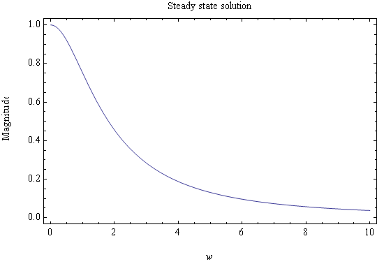
Solve for the forced response of a single-degree-of-freedom system to a harmonic excitation with \(\xi =1.1\) and \(\omega _{n}^{2}=4\). Plot the magnitude of the steady state response versus the driving frequency. For what values of \(\omega _{n}\) is the response maximum?
Answer Since the excitation is harmonic, assume it has the form \(F\sin \omega t\) where \(\omega \) is the deriving frequency. Then the equation of motion for the SDOF system is
\[ m\ddot{x}+c\dot{x}+kx=F\cos \omega t \]
Dividing by \(m\) and using \(\omega _{n}^{2}=\sqrt{\frac{k}{m}}\) and \(\xi =\frac{c}{c_{cr}}=\frac{c}{2\sqrt{km}}\) the above becomes\begin{equation} \ddot{x}+2\xi \omega _{n}\dot{x}+\omega _{n}^{2}x=f_{0}\cos \omega t \tag{1} \end{equation} Where \(f_{0}=\frac{F}{m}\)
Since this is an overdamped system (\(\xi >1\)), then the transient solution is \[ x_{h}\left ( t\right ) =e^{-\xi \omega _{n}t}\left ( Ae^{-\omega _{n}t\sqrt{\xi ^{2}-1}}+Be^{\omega _{n}t\sqrt{\xi ^{2}-1}}\right ) \] But we need only consider the particular solution since we are asked to plot the steady state solution. Assume \[ \fbox{$x_{p}\left ( t\right ) =c_{1}\cos \omega t+c_{2}\sin \omega t$}\] Then \begin{align*} \dot{x}_{p}\left ( t\right ) & =-\omega c_{1}\sin \omega t+c_{2}\omega \cos \omega t\\ \ddot{x}_{p}\left ( t\right ) & =-\omega ^{2}c_{1}\cos \omega t-c_{2}\omega ^{2}\sin \omega t \end{align*}
Substitute \(x_{p}\left ( t\right ) ,\dot{x}_{p}\left ( t\right ) ,\ddot{x}_{p}\left ( t\right ) \) in (1) we obtain\begin{align*} \left ( -\omega ^{2}c_{1}\cos \omega t-c_{2}\omega ^{2}\sin \omega t\right ) +2\xi \omega _{n}\left ( -\omega c_{1}\sin \omega t+c_{2}\omega \cos \omega t\right ) +\omega _{n}^{2}\left ( c_{1}\cos \omega t+c_{2}\sin \omega t\right ) & =f_{0}\cos \omega t\\ \left ( -c_{2}\omega ^{2}-2\xi \omega _{n}\omega c_{1}+c_{2}\omega _{n}^{2}\right ) \sin \omega t+\left ( -\omega ^{2}c_{1}+2\xi \omega _{n}c_{2}\omega +\omega _{n}^{2}c_{1}\right ) \cos \omega t & =f_{0}\cos \omega t \end{align*}
Hence by comparing coefficients in the LHS and RHS we obtain 2 equations to solve for \(c_{1}\) and \(c_{2}\) \begin{align*} -c_{2}\omega ^{2}-2\xi \omega _{n}\omega c_{1}+c_{2}\omega _{n}^{2} & =0\\ -\omega ^{2}c_{1}+2\xi \omega _{n}c_{2}\omega +\omega _{n}^{2}c_{1} & =f_{0} \end{align*}
or\begin{align} c_{1}\left ( -2\xi \omega _{n}\omega \right ) +c_{2}\left ( \omega _{n}^{2}-\omega ^{2}\right ) & =0\tag{2}\\ c_{1}\left ( \omega _{n}^{2}-\omega ^{2}\right ) +c_{2}\left ( 2\xi \omega _{n}\omega \right ) & =f_{0} \tag{3} \end{align}
From (2) we obtain \(c_{1}=\frac{c_{2}\left ( \omega _{n}^{2}-\omega ^{2}\right ) }{2\xi \omega _{n}\omega }\), and substitute this into (3)\begin{align*} \left ( \frac{c_{2}\left ( \omega _{n}^{2}-\omega ^{2}\right ) }{2\xi \omega _{n}\omega }\right ) \left ( \omega _{n}^{2}-\omega ^{2}\right ) +c_{2}\left ( 2\xi \omega _{n}\omega \right ) & =f_{0}\\ c_{2}\left [ \frac{\left ( \omega _{n}^{2}-\omega ^{2}\right ) ^{2}}{2\xi \omega _{n}\omega }+2\xi \omega _{n}\omega \right ] & =f_{0}\\ c_{2}\left [ \left ( \omega _{n}^{2}-\omega ^{2}\right ) ^{2}+4\xi ^{2}\omega _{n}^{2}\omega ^{2}\right ] & =2\xi \omega _{n}\omega f_{0} \end{align*}
Hence\[ \fbox{$c_{2}=\frac{2\xi \omega _{n}\omega f_{0}}{\left ( \omega _{n}^{2}-\omega ^{2}\right ) ^{2}+4\xi ^{2}\omega _{n}^{2}\omega ^{2}}$}\] Substitute the above into (2) we solve for \(c_{1}\)\[ c_{1}\left ( -2\xi \omega _{n}\omega \right ) +\left ( \frac{2\xi \omega _{n}\omega f_{0}}{\left ( \omega _{n}^{2}-\omega ^{2}\right ) ^{2}+4\xi ^{2}\omega _{n}^{2}\omega ^{2}}\right ) \left ( \omega _{n}^{2}-\omega ^{2}\right ) =0 \] or\[ \fbox{$c_{1}=\frac{f_{0}\left ( \omega _{n}^{2}-\omega ^{2}\right ) }{\left ( \omega _{n}^{2}-\omega ^{2}\right ) ^{2}+4\xi ^{2}\omega _{n}^{2}\omega ^{2}}$}\] Hence, since \[ x_{p}\left ( t\right ) =c_{1}\cos \omega t+c_{2}\sin \omega t \] Then\[ \fbox{$x_{p}\left ( t\right ) =\frac{f_{0}\left ( \omega _{n}^{2}-\omega ^{2}\right ) }{\left ( \omega _{n}^{2}-\omega ^{2}\right ) ^{2}+4\xi ^{2}\omega _{n}^{2}\omega ^{2}}\cos \omega t+\frac{2\xi \omega _{n}\omega f_{0}}{\left ( \omega _{n}^{2}-\omega ^{2}\right ) ^{2}+4\xi ^{2}\omega _{n}^{2}\omega ^{2}}\sin \omega t$}\]
We can convert the above to the form \(x_{p}\left ( t\right ) =c\cos \left ( \omega t-\theta \right ) \) by using the relation
\(c=\sqrt{c_{1}^{2}+c_{2}^{2}}\) and \(\tan \theta =\frac{c_{2}}{c_{1}}\), hence
\begin{align*} c & =\sqrt{\left ( \frac{f_{0}\left ( \omega _{n}^{2}-\omega ^{2}\right ) }{\left ( \omega _{n}^{2}-\omega ^{2}\right ) ^{2}+4\xi ^{2}\omega _{n}^{2}\omega ^{2}}\right ) ^{2}+\left ( \frac{2\xi \omega _{n}\omega f_{0}}{\left ( \omega _{n}^{2}-\omega ^{2}\right ) ^{2}+4\xi ^{2}\omega _{n}^{2}\omega ^{2}}\right ) ^{2}}\\ & =f_{0}\sqrt{\frac{\left ( \omega _{n}^{2}-\omega ^{2}\right ) ^{2}+4\xi ^{2}\omega _{n}^{2}\omega ^{2}}{\left ( \left ( \omega _{n}^{2}-\omega ^{2}\right ) ^{2}+4\xi ^{2}\omega _{n}^{2}\omega ^{2}\right ) ^{2}}}\\ & =\frac{f_{0}}{\sqrt{\left ( \omega _{n}^{2}-\omega ^{2}\right ) ^{2}+\left ( 2\xi \omega _{n}\omega \right ) ^{2}}} \end{align*}
The last equation can be written as
\begin{align*} c & =\frac{F/m}{\omega _{n}^{2}\sqrt{\left ( 1-\left ( \frac{\omega }{\omega _{n}}\right ) ^{2}\right ) ^{2}+\left ( 2\xi \frac{\omega }{\omega _{n}}\right ) ^{2}}}\\ & =\fbox{$\frac{F/k}{\sqrt{\left ( 1-\left ( \frac{\omega }{\omega _{n}}\right ) ^{2}\right ) ^{2}+\left ( 2\xi \frac{\omega }{\omega _{n}}\right ) ^{2}}}$} \end{align*}
And\begin{align*} \tan \theta & =\frac{c_{2}}{c_{1}}=\frac{\left ( \frac{2\xi \omega _{n}\omega f_{0}}{\left ( \omega _{n}^{2}-\omega ^{2}\right ) ^{2}+4\xi ^{2}\omega _{n}^{2}\omega ^{2}}\right ) }{\left ( \frac{f_{0}\left ( \omega _{n}^{2}-\omega ^{2}\right ) }{\left ( \omega _{n}^{2}-\omega ^{2}\right ) ^{2}+4\xi ^{2}\omega _{n}^{2}\omega ^{2}}\right ) }\\ & =\frac{2\xi \omega _{n}\omega }{\left ( \omega _{n}^{2}-\omega ^{2}\right ) }\\ & =\frac{2\xi \frac{\omega }{\omega _{n}}}{\left ( 1-\left ( \frac{\omega }{\omega _{n}}\right ) ^{2}\right ) } \end{align*}
Hence\begin{align} x_{p}\left ( t\right ) & =c\cos \left ( \omega t-\theta \right ) \nonumber \\ & =\overset{\text{magnitude}}{\overbrace{\frac{F/k}{\sqrt{\left ( 1-\left ( \frac{\omega }{\omega _{n}}\right ) ^{2}\right ) ^{2}+\left ( 2\xi \frac{\omega }{\omega _{n}}\right ) ^{2}}}}}\cos \left ( \omega t-\tan ^{-1}\left ( \frac{2\xi \frac{\omega }{\omega _{n}}}{\left ( 1-\left ( \frac{\omega }{\omega _{n}}\right ) ^{2}\right ) }\right ) \right ) \tag{4} \end{align}
Let \(r=\frac{\omega }{\omega _{n}}\), then the above becomes
\[ \fbox{$x_{p}\left ( t\right ) =\frac{F/k}{\sqrt{\left ( 1-r^{2}\right ) ^{2}+\left ( 2\xi r\right ) ^{2}}}\cos \left ( \omega t-\tan ^{-1}\left ( \frac{2\xi r}{\left ( 1-r^{2}\right ) }\right ) \right ) $}\]
For the supplied values for \(\omega _{n}^{2}=4\) and \(\xi =1.1\)then the above steady state solution becomes
\[ \fbox{$x_{p}\left ( t\right ) =\overset{X}{\overbrace{\frac{F/k}{\sqrt{\left ( 1-\frac{\omega ^{2}}{4}\right ) ^{2}+1.\,\allowbreak 21\omega ^{2}}}}}\cos \left ( \omega t-\tan ^{-1}\left ( \frac{1.1\omega }{\left ( 1-\frac{\omega ^{2}}{4}\right ) }\right ) \right ) $ }\]
To plot the magnitude, use a normalized \(F=1\), and let \(k=1\), use the supplied values for \(\omega _{n}^{2}=4\) and \(\xi =1.1\), hence magnitude \(X\) of steady state response is \[ X=\frac{1}{\sqrt{\left ( 1-\frac{\omega ^{2}}{4}\right ) ^{2}+1.\,\allowbreak 21\omega ^{2}}}\] Plot the expression for the magnitude \(X\) against the driving frequency \(\omega \)
To answer the final question about the resonance. Looking at the steady state solution in equation (4), we see that the amplitude of the \(x_{p}\) is \(\frac{F/k}{\sqrt{\left ( 1-\left ( \frac{\omega }{\omega _{n}}\right ) ^{2}\right ) ^{2}+\left ( 2\xi \frac{\omega }{\omega _{n}}\right ) ^{2}}}\) which is maximum when the denominator is minimum which occurs as \(\omega \) approaches \(\omega _{n}\), but in this problem since the system is overdamped, hence no oscillation will occur and the maximum response occurs when \(\omega =0\) (i.e. input is non oscillatory).
Discuss the stability of following system \(2\ddot{x}-3\dot{x}+8x=-3\dot{x}+\sin 2t\)
Answer
The system can be rewritten as
\[ 2\ddot{x}+8x=\sin 2t \]
We need to consider only the transient response (homogeneous solution). Hence the characteristic equation is
\[ 2\lambda ^{2}+8=0 \]
which has roots \(\pm \sqrt{2}j\). Since the roots are on the \(j\) axis, then this is a marginally unstable system
Calculate an allowable range of values for the gains \(K,g_{1},g_{2}\) for the system \(2\ddot{x}+0.8\dot{x}+8x=f\left ( t\right ) \) such that the closed-loop system is stable and the formulae for the overshoot and peak time of an underdamped system are valid
solution
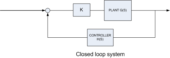
The transfer function of the controller (a P.D. controller) is \(H\left ( s\right ) =sg_{1}+g_{2}\) and for the plant (the system) the transfer function is \(G\left ( s\right ) =\frac{1}{2s^{2}+0.8s+8}\), hence the closed loop transfer function, which we call \(C\left ( s\right ) \), is \begin{align*} C\left ( s\right ) & =\frac{kG\left ( s\right ) }{1+H\left ( s\right ) KG\left ( s\right ) }\\ & =\frac{k\frac{1}{2s^{2}+0.8s+8}}{1+k\frac{sg_{1}+g_{2}}{2s^{2}+0.8s+8}}\\ & =\frac{k}{2s^{2}+0.8s+8+\left ( sg_{1}+g_{2}\right ) k}\\ & =\frac{k}{2s^{2}+\left ( 0.8+kg_{1}\right ) s+8+kg_{2}} \end{align*}
The characteristic equation is the denominator of the above transfer function. Hence
\[ f\left ( s\right ) =\overset{a}{\overbrace{2}}s^{2}+\overset{b}{\overbrace{\left ( 0.8+kg_{1}\right ) }}s+\overset{c}{\overbrace{8+kg_{2}}}\]
This has roots at\begin{align*} \lambda & =\frac{-b}{2a}\pm \frac{\sqrt{b^{2}-4ac}}{2a}\\ & =\frac{-0.8-kg_{1}}{4}\pm \frac{\sqrt{\left ( 0.8+kg_{1}\right ) ^{2}-8\left ( 8+kg_{2}\right ) }}{4}\\ & =-0.2-\frac{kg_{1}}{4}\pm \frac{\sqrt{k^{2}g_{1}^{2}+1.6kg_{1}-8kg_{2}-15.\,\allowbreak 36}}{4}\\ & =-0.2-\frac{kg_{1}}{4}\pm \sqrt{\frac{k^{2}g_{1}^{2}}{16}+0.1kg_{1}-0.5kg_{2}-0.96} \end{align*}
The system is stable if the real part of the roots is in the left hand side of the imaginary axis. Hence we require that \[ -0.2-\frac{kg_{1}}{4}<0 \]
Which implies \(\frac{-kg_{1}}{4}<0.2\) or \(\frac{kg_{1}}{4}>-0.2\) or \begin{equation} kg_{1}>-0.8 \tag{1} \end{equation}
and we require that \begin{equation} \frac{k^{2}g_{1}^{2}}{16}+0.1kg_{1}-0.5kg_{2}-0.96<0\tag{2} \end{equation}
Using the minimum value for \(kg_{1}\) which is \(-0.8\) and substitute that in above equation,
\begin{align*} \frac{0.8^{2}}{16}+0.1\left ( 0.8\right ) -0.5kg_{2}-0.96 & <0\\ 0.04+0.08-0.96-0.5kg_{2} & <0\\ -0.84-0.5kg_{2} & <0\\ -0.5kg_{2} & <0.84\\ 0.5kg_{2} & >-0.84 \end{align*}
Hence
\[ \fbox{$kg_{2}>-0.42$}\]
And \(k>0\) (positive gain is assumed). In summary, these are the allowed ranges
\begin{align*} kg_{2} & >-0.42\\ kg_{1} & >-0.8\\ \,k & >0 \end{align*}
Compute a feedback law with full state feedback (of the form given in equation 1.62 in the book that stabilizes the system \(4\ddot{x}+16x=0\) and causes the closed loop setting time to be 1 second.
Answer
Equation 1.62 in the book is
\[ m\ddot{x}+\left ( c+\bar{k}g_{1}\right ) \dot{x}+\left ( k+\bar{k}g_{2}\right ) x=\bar{k}f\left ( t\right ) \]
Notice that I modified the notation in this equation, where the lower case \(k\) is the stiffness and \(\bar{k}\) is the gain, this is to reduce ambiguity in notations
Using the controller required, the equation \(4\ddot{x}+16x=0\) becomes\[ m\ddot{x}+\bar{k}g_{1}\dot{x}+\left ( k+\bar{k}g_{2}\right ) x=0 \]
Notice that there is no damping in \(4\ddot{x}+16x=0\), (\(c=0\)), but now \(\bar{k}g_{1}\)term acts in place of the damping. From the original equation \(m=4\) and \(k=16\), hence we can write the above as
\[ 4\ddot{x}+\bar{k}g_{1}\dot{x}+\left ( 16+\bar{k}g_{2}\right ) x=0 \] The characteristic equation is \[ 4\lambda ^{2}+\bar{k}g_{1}\lambda +\left ( 16+\bar{k}g_{2}\right ) =0 \] Hence\begin{align*} \lambda _{1,2} & =\frac{-b\pm \sqrt{b^{2}-4ac}}{2a}=\frac{-\bar{k}g_{1}\pm \sqrt{\left ( \bar{k}g_{1}\right ) ^{2}-16\left ( 16+\bar{k}g_{2}\right ) }}{8}\\ & =\frac{-\bar{k}g_{1}}{8}\pm \frac{1}{8}\sqrt{\bar{k}^{2}g_{1}^{2}-256-16\bar{k}g_{2}} \end{align*}
Hence for stability, the real part of the root must be negative, hence \(\frac{-\bar{k}g_{1}}{8}<0\) or \(\frac{\bar{k}g_{1}}{8}>0\) or \(\bar{k}g_{1}>0\)
And we require that \(\bar{k}^{2}g_{1}^{2}-256-16\bar{k}g_{2}<0\) (for oscillation to occur). This implies\begin{equation} \bar{k}^{2}g_{1}^{2}-16\bar{k}g_{2}<256 \tag{1} \end{equation} Now settling time is given by\[ t_{s}=\frac{3.2}{\omega _{n}\zeta }=\frac{3.2}{\omega _{n}\frac{c}{c_{cr}}}=\frac{3.2}{\omega _{n}\frac{c}{2\omega _{n}m}}=\frac{3.2\left ( 2m\right ) }{c}\] But in this system (modified) \(m=4\) and \(c=\bar{k}g_{1}\), hence the above becomes\[ t_{s}=\frac{3.2\times 8}{\bar{k}g_{1}}\] But \(t_{s}=1\)sec., hence\[ \fbox{$\bar{k}g_{1}=25.\,\allowbreak 6$}\] Substitute the above into (1) we obtain\begin{align*} 25.\,\allowbreak 6^{2}-16\ \bar{k}g_{2} & <256\\ 655.\,\allowbreak 36-16\ \bar{k}g_{2} & <256\\ 2.\,\allowbreak 56-0.062\,5\ \bar{k}g_{2} & <1\\ -0.062\,5\ \bar{k}g_{2} & <-1.56\\ \bar{k}g_{2} & >\frac{1.56}{0.062\,5} \end{align*}
Hence
\[ \fbox{$\bar{k}g_{2}>24.\,\allowbreak 96$}\]
To plot the solution, choose \(\bar{k}g_{2}\) say\(100\) and since \(\bar{k}g_{1}=25.6\), then since the loop back equation of motion is
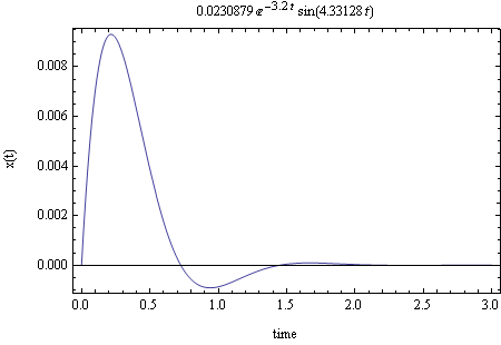
\[ m\ddot{x}+\bar{k}g_{1}\dot{x}+\left ( k+\bar{k}g_{2}\right ) x=0 \] Then plugging in the above values for \(\bar{k}g_{2}\) and \(\bar{k}g_{1}\) we obtain \begin{align*} 4\ddot{x}+25.6\dot{x}+\left ( 16+100\right ) x & =0\\ 4\ddot{x}+25.6\dot{x}+116x & =0 \end{align*}
To confirm the result, I plot the solution to the above equation (which is now stable) using some initial condition such as \(v_{0}=0.5\) and \(x_{0}=0\) (arbitrary I.C.). The result is the following
Find the equilibrium points of the nonlinear pendulum equation \(ml^{2}\ddot{\theta }+mgl\sin \theta =0\)
Answer
The equation of motion can be simplified to be\[ \ddot{\theta }+\frac{g}{l}\sin \theta =0 \] Convert to state space format.\[\begin{bmatrix} x_{1}=\theta \\ x_{2}=\dot{\theta }\end{bmatrix} \rightarrow \begin{bmatrix} \dot{x}_{1}=\dot{\theta }=x_{2}\\ \dot{x}_{2}=\ddot{\theta }=-\frac{g}{l}\sin \theta =-\frac{g}{l}\sin x_{1}\end{bmatrix} \] Hence\[ \overset{\dot{X}}{\overbrace{\begin{bmatrix} \dot{x}_{1}\\ \dot{x}_{2}\end{bmatrix} }}=\begin{bmatrix} x_{2}\\ -\frac{g}{l}\sin x_{1}\end{bmatrix} \]
For equilibrium of a nonlinear system, we require that \(\dot{X}=0\), hence \(x_{2}=0\) and \(-\frac{g}{l}\sin x_{1}=0\)
But \(-\frac{g}{l}\sin x_{1}=0\) implies that \(x_{1}=n\pi \) for \(n=0,\pm 1,\pm 2,\cdots \)
Since \(x_{1}=\theta \) , and \(\theta \) is assumed to be zero when the pendulum is hanging in the vertical direction. Hence the equilibrium positions are as shown below (showing the first stable and the first unstable points)
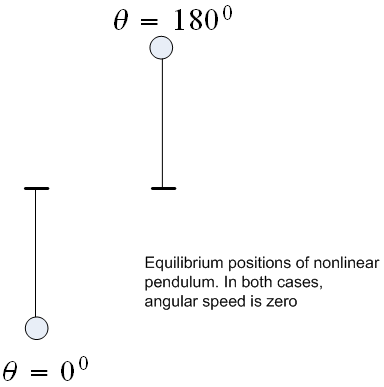
In both cases, \(\dot{\theta }=0\). Notice that at \(\theta =n\pi \) for \(n=\pm 1,\pm 3,\pm 5,\cdots \) the pendulum in a marginally stable equilibrium position, while at \(n=0,\pm 2,\pm 4,\cdots \) it is at a stable equilibrium position.