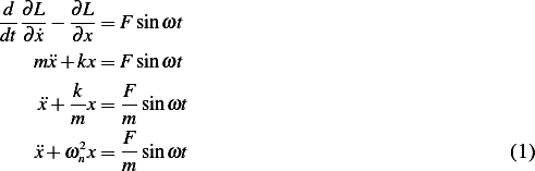
Solution sketch: Obtain the Lagrangian, find EQM, solve in terms of general initial conditions  and
and
 , then solve parts (a) and (b) using this general solution.
This is one degree of freedom system. Using  as the generalized coordinates, we first obtain the
Lagrangian
as the generalized coordinates, we first obtain the
Lagrangian 

Where
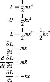
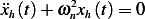
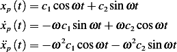
Hence the EQM is (using the Lagrangian equation), and  and
and  rad/sec. (the forcing
frequency)
rad/sec. (the forcing
frequency)
Where  . The solution is
 | (2) |
To obtain 
Assume  and substitute in the above ODE we obtain the characteristic equation
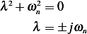
Hence
 | (3) |
Guess
Notice, the above guess is valid only under the condition that  which is the case in this problem.
Now, substitute the above 3 equations into (1) we obtain
which is the case in this problem.
Now, substitute the above 3 equations into (1) we obtain
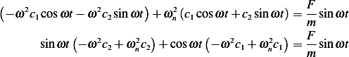
By comparing coefficients, we obtain
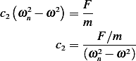
and  , hence
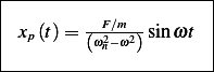
Then from (2) we obtain
Using (3) in the above
 | (4) |
Now assume  and
and  For the condition
  we obtain

For the condition  we obtain
Hence
Hence (4) can be written as

Let  , the above becomes

But  hence
hence
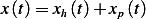
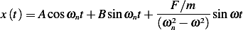
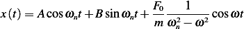
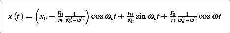
Therefore, the general solution is
 | (5) |
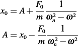
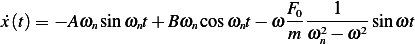
When  we obtain from (5)
 | (6) |
Substitute numerical values, and plot the solution.  rad/sec.
 then equation (6) becomes
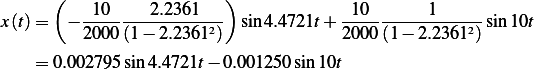
In the following plot, we show the homogeneous solution and the particular solution separately, then show the general solution.
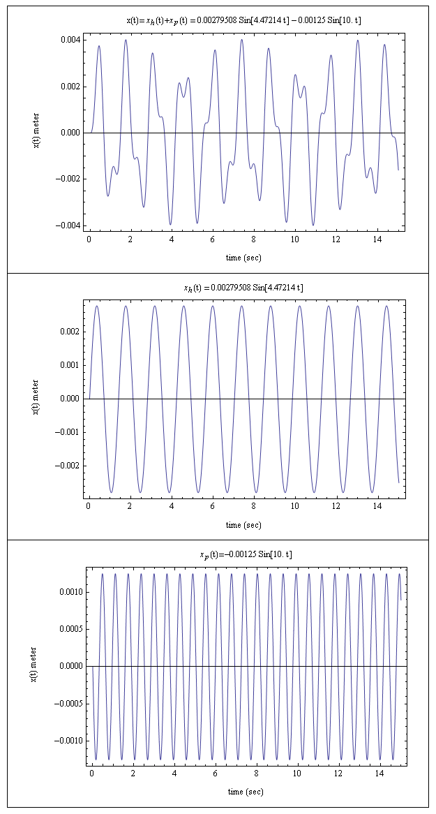
When  and
and  we obtain from (5)

Substitute numerical values found in part(a), then the solution becomes
In the following plot, we show the homogeneous solution and the particular solution separately, then show the general solution.

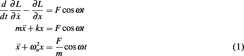
Following the approach taken in problem 2.7, the EQM is
And  where
where  . For
. For  guess
guess  and
following the same steps in problem 2.7, we obtain
and
following the same steps in problem 2.7, we obtain

Notice that the above guess is valid only under the condition that  . Compare coefficients, we find
 and
and
Hence
Then, the general solution is
 | (1) |
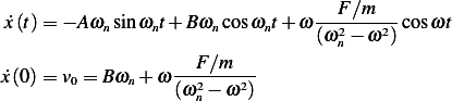
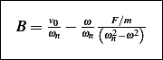
Let, at  ,
,  , and
, and  ,then from (1), we find
And since
Then

Therefore, the general solution is (from (1))
To make the response oscillate at frequency  only, we can set
  to eliminate the
  , and set
 to eliminate the
  term. Hence, the initial conditions are
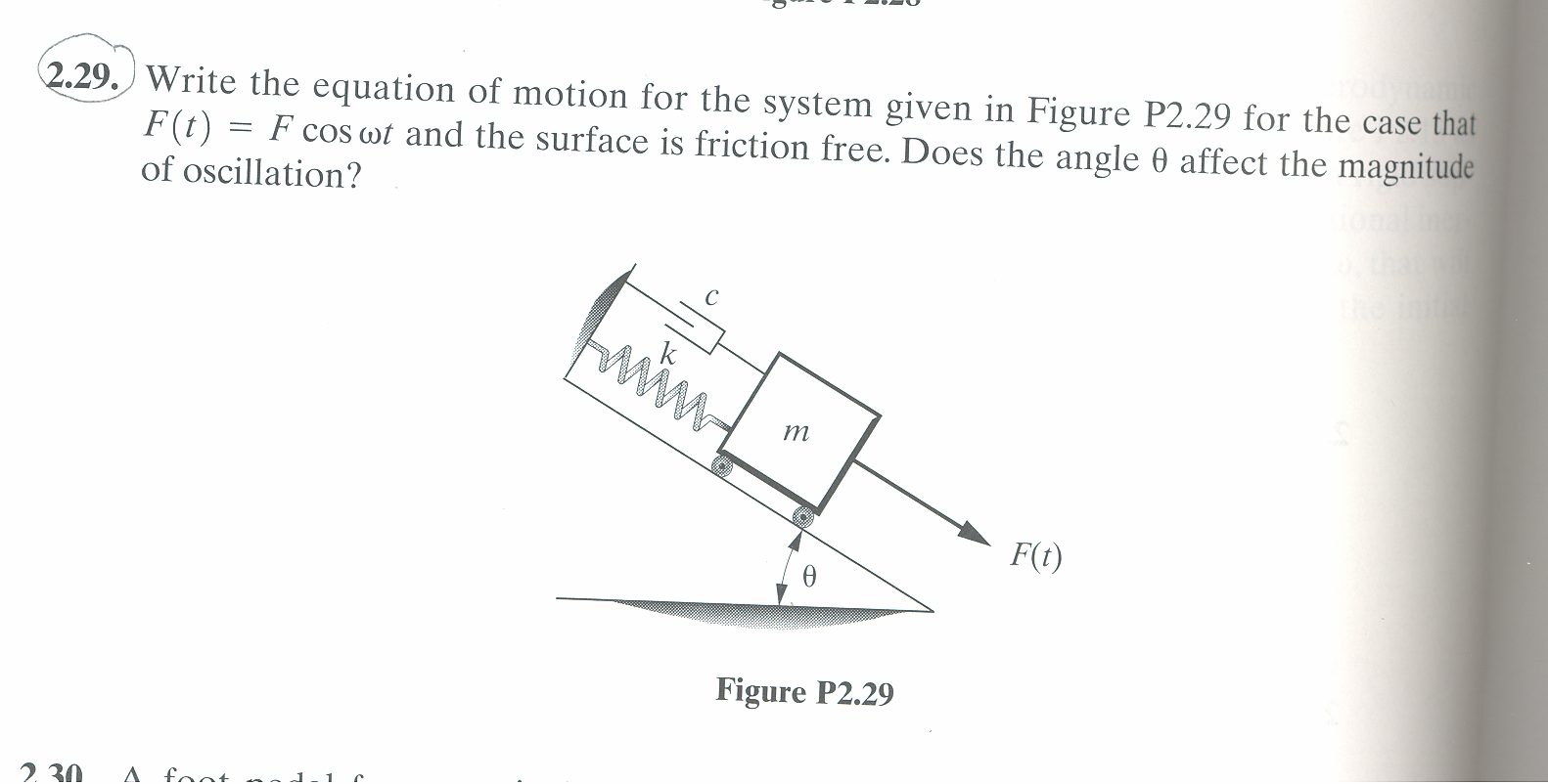
This is one degree of freedom system. Using  along the inclined surface as the generalized coordinates, we first
obtain the Lagrangian
along the inclined surface as the generalized coordinates, we first
obtain the Lagrangian 
We first note that 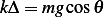 and the mass will lose potential as it slides down the surface. We measure
everything from the relaxed position (not the static equilibrium.) This is done to show more clearly that the
angle do not affect the solution.
and the mass will lose potential as it slides down the surface. We measure
everything from the relaxed position (not the static equilibrium.) This is done to show more clearly that the
angle do not affect the solution.

Where
Hence
But  , hence the above reduces to

Hence the EQM is (using the Lagrangian equation)
Where  . We see that the angle
  is not in the EQM. Hence the solution does not involve
  and
the oscillation magnitude is not affected by the angle. Intuitively, the reason for this is because the angle effect
is already counted for to reach the static equilibrium. Once the system is in static equilibrium, the angle no
longer matters as far as the solution is concerned.
and
the oscillation magnitude is not affected by the angle. Intuitively, the reason for this is because the angle effect
is already counted for to reach the static equilibrium. Once the system is in static equilibrium, the angle no
longer matters as far as the solution is concerned.
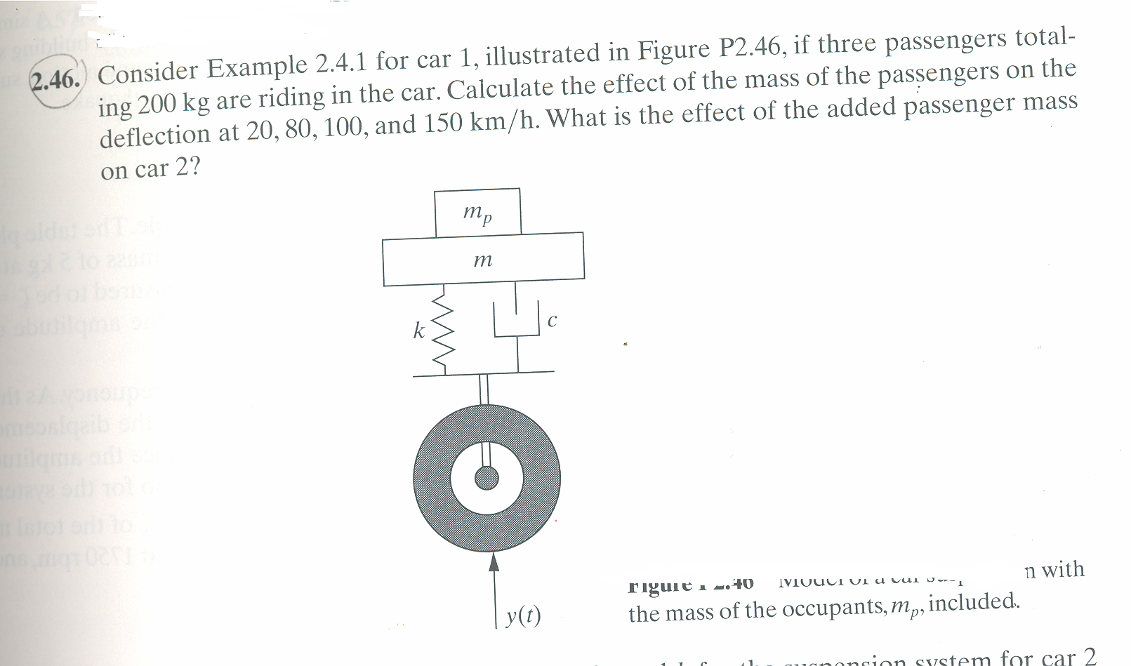
From example 2.4.1, we note the following table
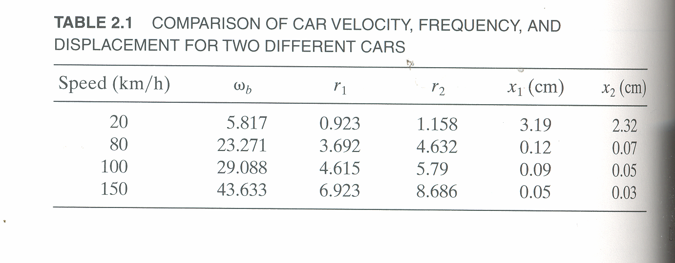
Also, from example 2.4.1, the mass of car 1 is  and the mass of car 2 is
  . Hence we
write
. Hence we
write

To find the deflection of the car, we use equation 2.70 in the book, which is
Where  is the magnitude of the steady state deflection and
  is the magnitude of the base deflection, which
is given as
is the magnitude of the base deflection, which
is given as  meters in the example.
Hence, for each speed, we calculate  and then we find
  and then find
  and then find
 and then using equation(1), we calculate
  . This is done for each different speed (all for car
 Next, we do the same for car
  . These calculation are shown in the following table. Note also that
 N s/m as given in the example and
  N/m
N/m
car 1
 |  |  |  |  |  |
 |  |  |  |  |  |
 |  |  |  |  |  |
 |  |  |  |  |  |
 |  |  |  |  |  |
 |  |  |  |  |  |
 |  |  |  |  |  |
 |  |  |  |  |  |
 |  |  |  |  |  |
 |  |  |  |  |  |
 values) for all speeds. Adding passengers,
causes
values) for all speeds. Adding passengers,
causes  to change. This results in making the deflection smaller when passengers are in the car as compared
without them. Heaver cars and heavier passenger results in smaller deflection values. For the lighter car
however, adding the passenger did not result in smaller deflection for all speeds. For speed
to change. This results in making the deflection smaller when passengers are in the car as compared
without them. Heaver cars and heavier passenger results in smaller deflection values. For the lighter car
however, adding the passenger did not result in smaller deflection for all speeds. For speed  , adding the
passenger caused a larger defection (
, adding the
passenger caused a larger defection ( vs.
vs.  ). As car 1 speed became larger, the deflection became
smaller for both cars.
). As car 1 speed became larger, the deflection became
smaller for both cars.
So, in conclusion: lighter cars have larger deflections at bumps, and the faster the car, the smaller the deflection.
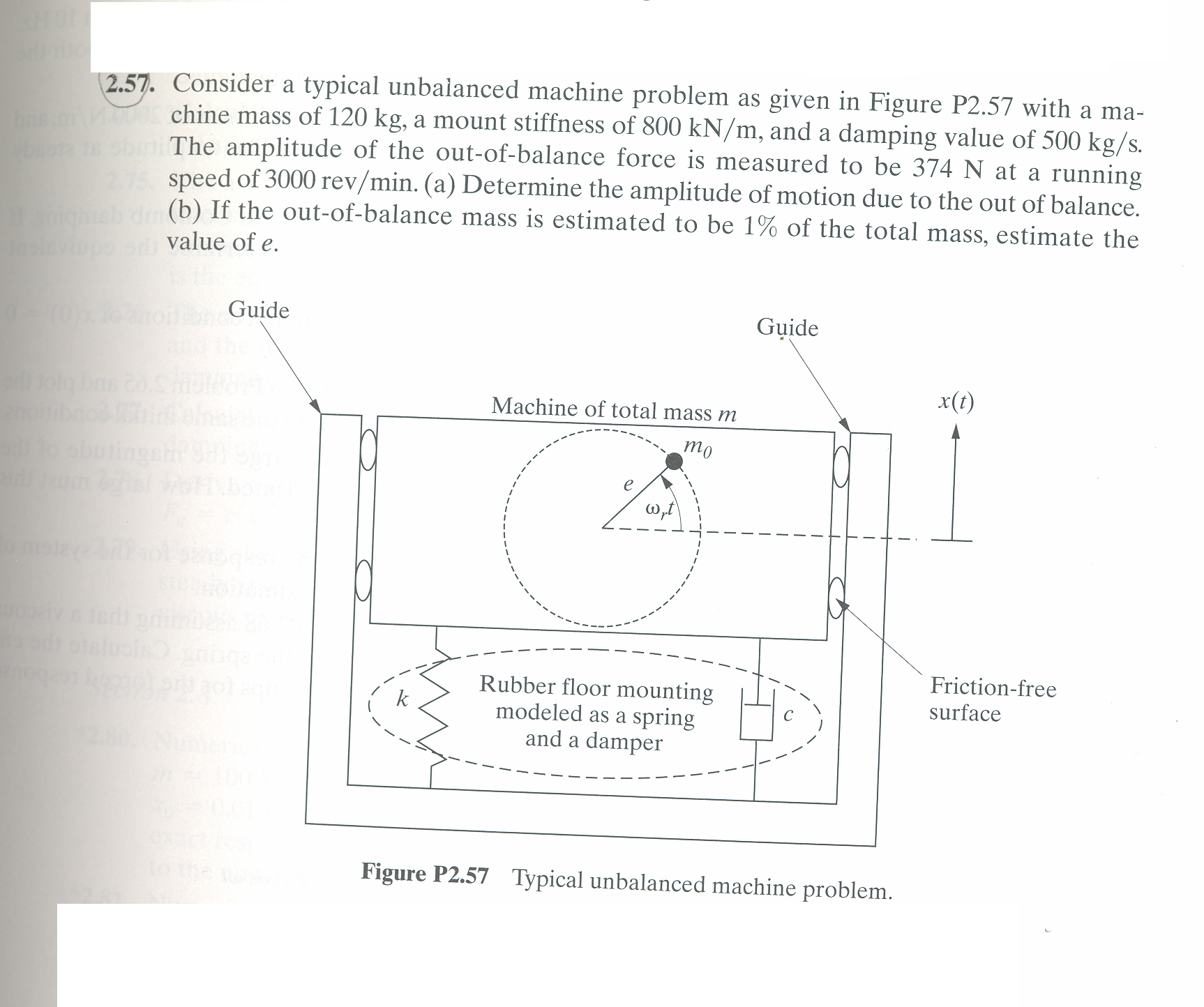
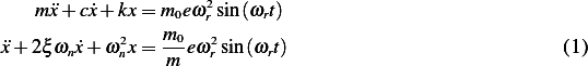
Given  N/M,
N/M,  kg/s, and mass
  has angular speed of
 radians per seconds
The rotating mass will cause a downward force as the result of the centripetal force  . Hence the
reaction to this force on the machine will be in the upward direction. Hence
. Hence the
reaction to this force on the machine will be in the upward direction. Hence
Hence the machine equation of motion is
By guessing 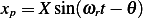 then we find that (The method of undetermined coefficients is used,
derivation is show in text book at page 115)
then we find that (The method of undetermined coefficients is used,
derivation is show in text book at page 115)
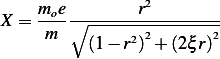 | (2) |
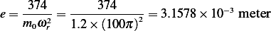
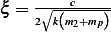
This is the maximum magnitude of motion in steady state. In the above,  . Hence to find
  we
substitute the given values in the above expression. We first note that we are told that
we
substitute the given values in the above expression. We first note that we are told that  , hence
 but we found that
  rad/sec, hence
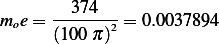
And
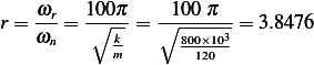
And
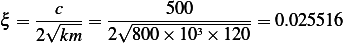
Substitute into (2) we obtain
We are told that  , hence
  . And since we are told that
  ,
then
,
then