HW Math 504. Spring 2008. CSUF
Problems 10.5 and 10.6
by Nasser Abbasi
Problem 10.5
Solution
|
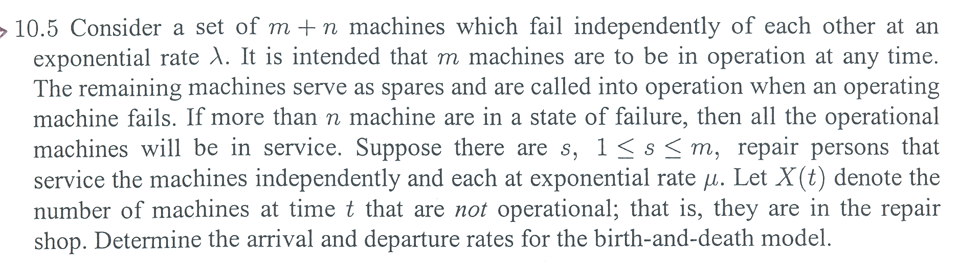
Illustrating model diagram
for problem 10.5
|
In the above,
 is the number of broken machines in the queue.
 is maximum capacity of the operating room. The goal is to keep this room
filled to its capacity. In other words, to keep
is maximum capacity of the operating room. The goal is to keep this room
filled to its capacity. In other words, to keep
 machines in operations.
 is the capacity of the spare room.
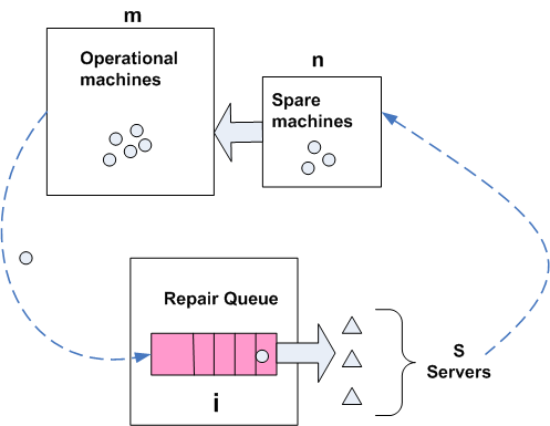
Calculating arrival rates:
Need to determine
 This can happen when one machine fails, but no server completes its service
meanwhile. Hence we do not need to consider the servers part in this analysis.
There are 2 cases to consider:
This can happen when one machine fails, but no server completes its service
meanwhile. Hence we do not need to consider the servers part in this analysis.
There are 2 cases to consider:
-
 (there are
 machines in
operations)
machines in
operations)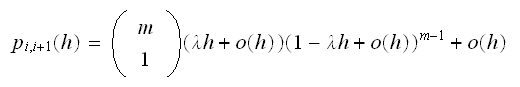 In the above, the last term
 accounts for other possible conditions under which
 can increase by one but which is considered to be less likely, such as 2
machines break down and one server completes its service.
can increase by one but which is considered to be less likely, such as 2
machines break down and one server completes its service.
In the above,
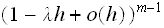 simplifies to zero when
 is very small, hence the above equation becomes
 Comparing the above with the Hence we see
 we see
that
we see
that or in other words,
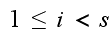
-
 (there are less than
 machines in
operations)
machines in
operations)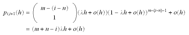 Hence we see that
 or in other words,
Calculating departure rates:
Need to determine
 ,
this can happen when a server completes its job but no machine fails
meanwhile, Hence we only need to consider the servers. There are 2 cases to
consider:
,
this can happen when a server completes its job but no machine fails
meanwhile, Hence we only need to consider the servers. There are 2 cases to
consider:
-
 (Queue is empty and not all servers at working on fixing machines at
hand)
(Queue is empty and not all servers at working on fixing machines at
hand)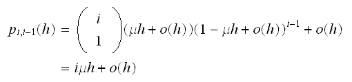
Hence
 ,
or since this is a birth/death process, we write
,
or since this is a birth/death process, we write
-
 (All servers at
busy)
(All servers at
busy)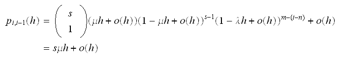
Hence
 ,
Hence
,
Hence
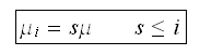
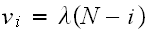
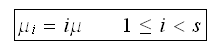
Therefore, we summarize all the above as follows

Departure rate

for
and

for

Notice that
arrival rate does not depend on the number of
servers

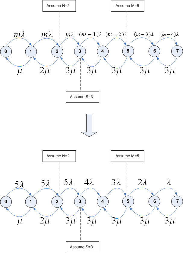
The following state transition diagram illustrates the above result, with
arrows leaving/entering states show the rate of arrival and departure on them
per the above result. To make the diagram easier to make, I assume the
following values:
Notice that
 and
and
 as
expected.
as
expected.
Now
compute the steady state distribution
 (This is not asked for in this problem, but need to do this to solve problem
12.3 later on and implement it)
(This is not asked for in this problem, but need to do this to solve problem
12.3 later on and implement it)
Starting with the balance equation, where to balance the rate out of a state,
with the rate into a state. We have
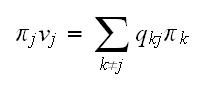
Hence for state
 we have
But
 and
and
 hence
hence
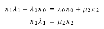
For state
 we have
but
 ,
,
 hence
the above becomes
hence
the above becomes
But from (1) we have
 ,
hence the above becomes
,
hence the above becomes
Continue this way, we obtain that

From the above, if we solve in terms of
 we obtain that
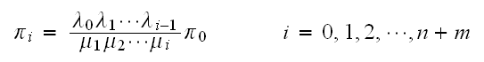
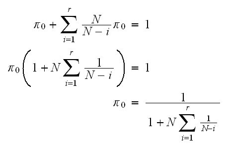
and with the equation
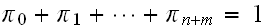 we can now solve for all
 as follows
Hence
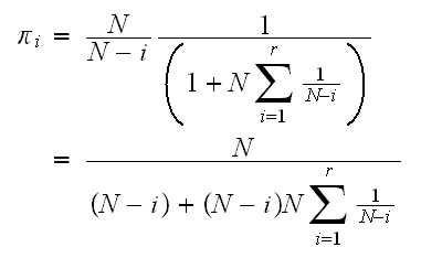
Now that
 is found, we can find the remaining
 using (3)
Problem 10.6
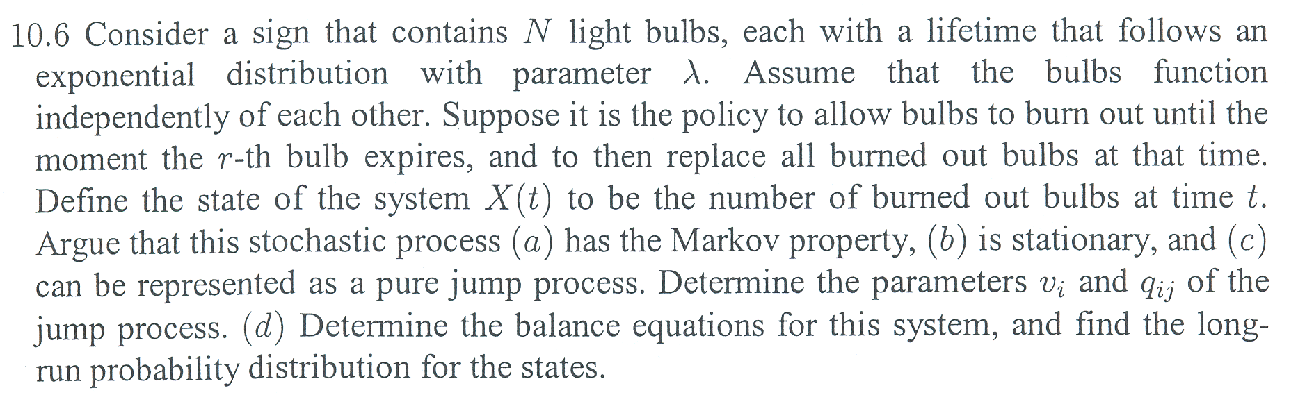
Review
of the problem setup: Imagine there is a queue of length
 .
Burned out bulbs enter the queue (with inter-arrival time which is a random
variable distributed as an exponential with rate
.
Burned out bulbs enter the queue (with inter-arrival time which is a random
variable distributed as an exponential with rate
 ).
Bulbs continue to enter the queue until the queue is full, then at that moment
we imagine a single server processing the bulbs in the queue all at once and
immediately all
).
Bulbs continue to enter the queue until the queue is full, then at that moment
we imagine a single server processing the bulbs in the queue all at once and
immediately all
 bulbs become operational again and the queue is now empty. This process
repeats again and again.
bulbs become operational again and the queue is now empty. This process
repeats again and again.
Part A
A stochastic process
 is defined to have the Markov property if its transition to the next state
depends only on the current state and not on any earlier states. In other
words it satisfies the
following
is defined to have the Markov property if its transition to the next state
depends only on the current state and not on any earlier states. In other
words it satisfies the
following In this problem
 is the number of burned out bulbs in the queue at any time
 .
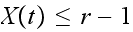
When
.
When
 then
then
 can be viewed as a counting process (or pure birth process) or a Poisson
process (until the queue become full).
can be viewed as a counting process (or pure birth process) or a Poisson
process (until the queue become full).
Therefore, The time between each successive events (where an event causes the
count to increase by one) is a random variable with exponential distribution
(we are also given this fact in the problem). But the exponential distribution
is
memoryless Note_1
by definition. Therefore it does not depend on clock time but only on the
length of the time interval. Hence the process satisfies the Markov property.
part
B
A stochastic process
 is defined to be
stationary Note_2
if its state transition
is defined to be
stationary Note_2
if its state transition
 do not depend on when the transitions happen but only on the time interval
 .
In other words, random process
.
In other words, random process
 is stationary if
 For any
 So, letting
 ,
the system is stationary
if
,
the system is stationary
if This process is clearly stationary, since it is a counting process (when
 ).
A counting Poisson process is stationary since it does not depend on clock
time as was argued in part (A). To show this more clearly, since this is a
counting process, then by definition of the Poisson
process
).
A counting Poisson process is stationary since it does not depend on clock
time as was argued in part (A). To show this more clearly, since this is a
counting process, then by definition of the Poisson
process We see that the probability of
 does not depend on
 and depends only on the time interval
 .
If this was a non-stationary process, then
.
If this was a non-stationary process, then
 would appear in the RHS above. I.e. the probability of the random variable
would depend on clock time, but we see from the above definition that it does
not.
would appear in the RHS above. I.e. the probability of the random variable
would depend on clock time, but we see from the above definition that it does
not.
Part(c)
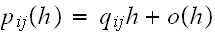
A stochastic process is a pure jump process if the transition probabilities
can be written as
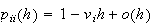 and
and
 as
as

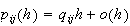
In this problem
 is the probability than no bulb burns out during an interval
 .
This is given by the probability than no bulb burns out from the current
number of functional bulbs which is
.
This is given by the probability than no bulb burns out from the current
number of functional bulbs which is
 .
Due to independence, we obtain
.
Due to independence, we obtain
Applying Binomial expansion
 ,
to the above, and taking
,
to the above, and taking
 we
obtain
we
obtain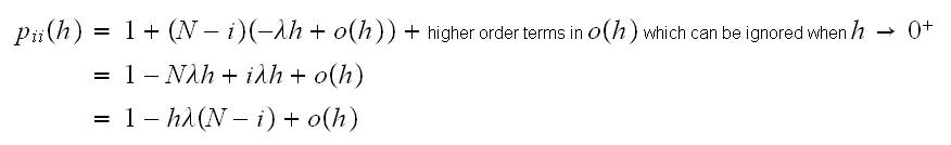 Hence we can write
 where
where
Now
 is the probability that there will be
 failed bulbs after
 units of time given that there is already
 failed bulbs. For this to occur, then we need to have
 bulbs fail in
 units of time. We can solve for the general case when
 but
since we will let
but
since we will let
 it
is most likely that there will be only one event occur (one bulb fail) during
this time, and we can collect all other less likely probabilities in the
it
is most likely that there will be only one event occur (one bulb fail) during
this time, and we can collect all other less likely probabilities in the
 term. Hence we will only consider
 in
the
following.
in
the
following.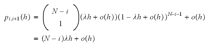
Therefore from
 we see that
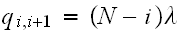 i.e.
i.e.
Hence the
 matrix (The rate matrix)
is
matrix (The rate matrix)
is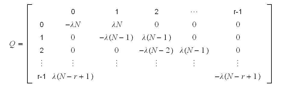
Part (d)
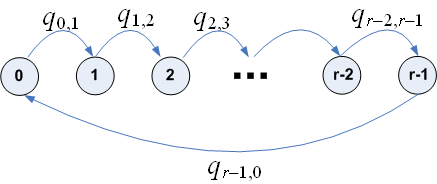
|
rate flow diagram for problem
10.6
|
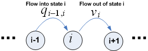
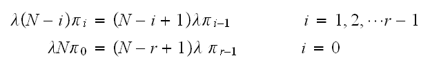
The balance equation can be obtained from balancing the flow out rate of a
state
 (which is given by
 )
by all the flow in rate into the state which is given by
)
by all the flow in rate into the state which is given by
 as illustrated below for the above problem
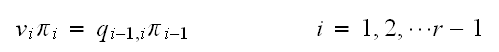
Hence we write
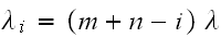
and for state
 we have
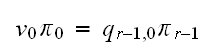
Therefore we obtain
Hence we have for
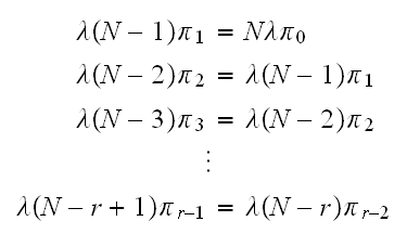
Therefore we have
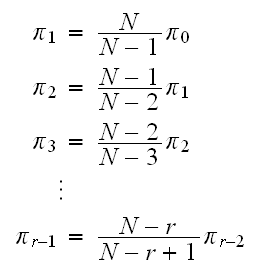
back substitute, we obtain
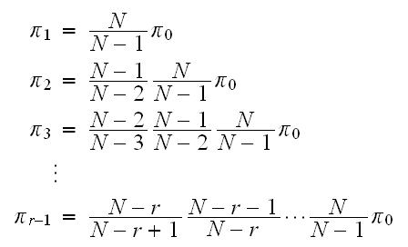
Hence
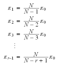
We notice that the last equation above, is the same as for the case
 .
Hence we have one of the
.
Hence we have one of the
 equations duplicated. Hence we need one more equation to solve for the
unknowns
equations duplicated. Hence we need one more equation to solve for the
unknowns
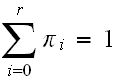
 and for that we use
Therefore, the general expression for
 is
is
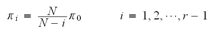
Now since
 ,
then we write
,
then we write
So now that we know
 from (2), we substitute it into (1) and solve for the remaining

But
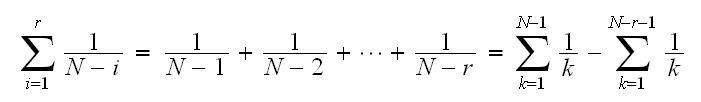
Which is the difference between 2 partial sums of harmonic numbers. Let
 ,
then
,
then
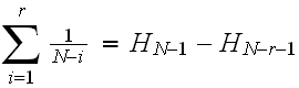 hence (3) becomes
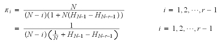
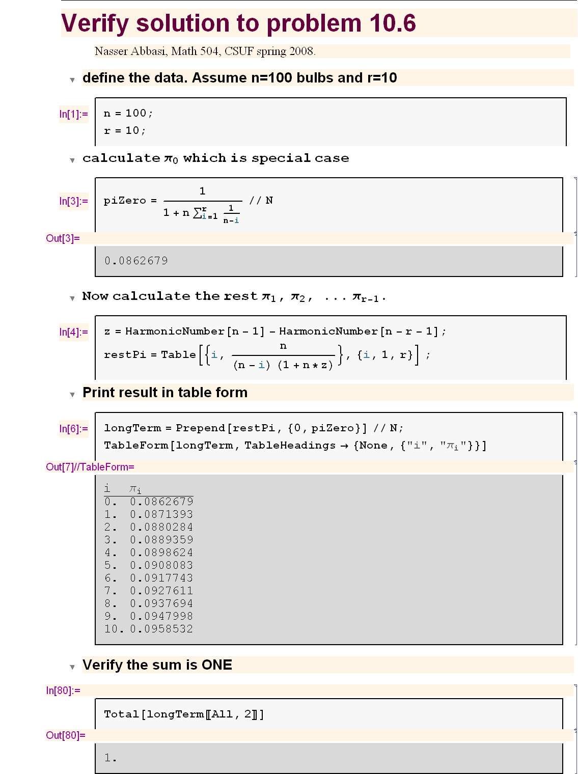
Hence
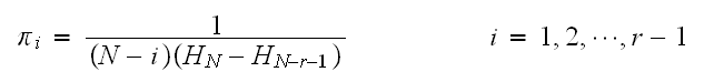
This is a small program which show the long term
 for
for
 using the above equation