Limiting process for Einstein-Wiener random walk simulation. Computer assignment #2, Math 504, CSUF, spring 2008
by Nasser Abbasi
\clearpage
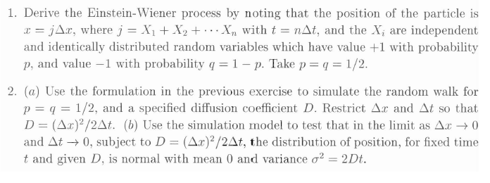
We are solving problem #2 as described in the following screen shot (taken from the class handout)
Short background on the problem: In this project we are asked to verify an analytical result derived in a handout given in the class called 'Continuos approximation to random walk'.
A random walk is formulated, by proposing that
 which
is the probability that the position of a particle at
which
is the probability that the position of a particle at
 and at time
 can be expressed as
 ,
where
,
where
 represents a density per unit length, which gives a measure of the particle
being at that position
represents a density per unit length, which gives a measure of the particle
being at that position
 at time

Starting with this and applying a limiting argument lead to a partial
differential equation whose solution is the normal distribution function with
certain mean and variance. However, the condition for arriving at the PDE was
that as we make
 and
and
 small, we needed to keep the ratio
 constant.
In this assignment, we simulate a random walk as
 and
and
 are made smaller and smaller subject to this same condition to verify if the
distribution of the final position of the random walk converges to the
solution of the PDE which is normal distribution and if the converged
distribution will have the same variance of
are made smaller and smaller subject to this same condition to verify if the
distribution of the final position of the random walk converges to the
solution of the PDE which is normal distribution and if the converged
distribution will have the same variance of
 and same mean of
 as does the solution of the PDE.
The details of the theoretical derivation is shown in the above mentioned handout. A diagram below is made to help illustrate the overall purpose of this assignment. In this assignment, we are working on the flow shown on the right side below.
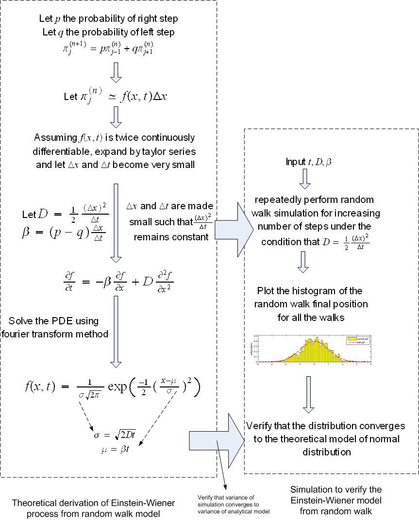
Random walk simulation to
verify the Einstein-Wiener analytical derivation
These are the questions we are trying to answer in this project
Does the distribution of the random walk final position generated by
increasing the number of steps for fixed
 (total time of the random walk) while keeping the ratio
 constant
(equal to
constant
(equal to
 ),
converges to a normal distribution (which is the solution of the
Einstein-Wiener process model)?
),
converges to a normal distribution (which is the solution of the
Einstein-Wiener process model)?
Does the variance of the above distribution converges, as
 and
and
 under the above mentioned condition of keeping
 to the analytical variance of
 and the theoretical mean of
 ?
?
The input to the program is
 where
where
 is the total random walk time and
 represents
the terms as shown in the diagram above.
represents
the terms as shown in the diagram above.
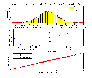
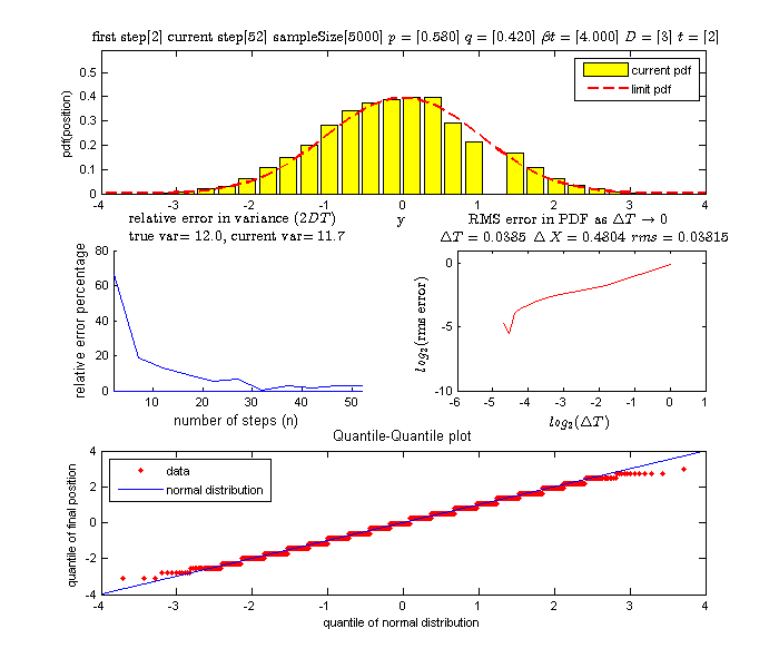
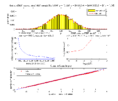
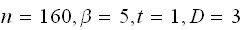
A distribution of the final random walk position is generated by running the random walk simulation a number of times (called the sample size). In each such run, we use a specific number of steps. The number of steps is increased, and we generate another distribution. We keep doing this and plot each distribution as the number of steps is increased.
At the end of the simulation, to verify that the distribution in the limit is normal. A quantile-quantile plot is made to compare the generated histogram with the theoretical standard normal distribution to see if the result is close to a straight line or not. Also a plot is made showing the convergence of the variance of the current distribution as number of steps is increased by keeping track of the relative error in the variance. In addition, the RMS error between the standard normal and the current distribution is calculated and plotted as a function of delta(T) as delta(T) is made smaller and smaller. The program is written in Matlab version 2007a and uses the statistics toolbox.
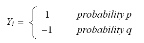
We simulate a random walk, where each step made is either to the left or to
the right with probability
 and
and
 respectively.
Let
 be either
 or
or
 depending if we make a right or a left step. Hence
 and now if we let
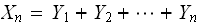 then the final position of the random walk can be written
as
then the final position of the random walk can be written
as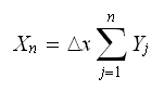
where
 is the step size. The step size is found by solving
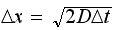 where
where
 is the diffusion parameter which is an input, and
 is the current time step found by dividing the total simulation fixed time
 ,
which is an input, by the current number of steps
,
which is an input, by the current number of steps
 .
.

This program handles a general value for
 other than zero. To be able to accomplish this, we need to determine the
correct starting step size
other than zero. To be able to accomplish this, we need to determine the
correct starting step size
 to avoid the problem with coming up with a value for the probability
 being larger than
 .
So, this was done in the initialization stage using this formula
.
So, this was done in the initialization stage using this formula
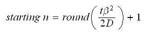
And the simulation was started from the above
 and not from
 .
.
To answer the first question of this simulation, which is to determine if the
final position distribution converges to normal distribution with mean
 and variance
 ,
a quantile plot was used. In this plot, the quantile for the standard normal
distribution was plotted against the quantile of the distribution of the final
position.
,
a quantile plot was used. In this plot, the quantile for the standard normal
distribution was plotted against the quantile of the distribution of the final
position.
The
 of the quantile-quantile plot was found as follows
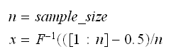
Where
 is the inverse of the CDF for the standard normal distribution (the matlab
function norminv() was used for this). While the
is the inverse of the CDF for the standard normal distribution (the matlab
function norminv() was used for this). While the
 is the quantile of the actual data (the sample data of the final distribution
of the random walk position). This was found by sorting the data from small to
large and then using the resulting sorted vector as the
is the quantile of the actual data (the sample data of the final distribution
of the random walk position). This was found by sorting the data from small to
large and then using the resulting sorted vector as the
 values. Notice that the distribution was already standardized using
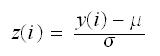
Where
 and
and
 ,
,
A number of experiments were performed for different input parameters. The table below lists the variance of the distribution of the final position as the number of steps is increased. The run parameters are also shown
starting step
number ,
,

sample size
 number of bins
 seed
seed
 (number of steps)
 |
Variance | True variance (2Dt) |  |
 |
 |
 |
 |
 |
 |
 |
 |
 |
 |
 |
 |
 |
 |
 |
 |
 |
 |
 |
 |
 |
 |
 |
 |
 |
 |
 |
 |
 |
 |
 |
 |
 |
 |
 |
 |
 |
 |
 |
 |
 |
 |
 |
 |
 |
 |
 |
 |
 |
 |
 |
 |
 |
 |
 |
 |
 |
 |
 |
 |
 |
 |
 |
 |
Since the parameters
 ,
then running for
,
then running for
 will produce the same numerical values already contained in the first
experiment when looking at the table above up to
will produce the same numerical values already contained in the first
experiment when looking at the table above up to
 (the
program starts by seeding the random number generator, so nothing will change
here and we will just produce a subset of the result already produced in first
experiment). So I will just show the final plot, showing the convergence of
the histogram and the quantile-quantile plot
(the
program starts by seeding the random number generator, so nothing will change
here and we will just produce a subset of the result already produced in first
experiment). So I will just show the final plot, showing the convergence of
the histogram and the quantile-quantile plot
Again, as described at the start of experiment 2 above, this is a subset of the first experiment. We will show the final plot only to show how close to the standard normal the final position histogram is.

The following 2 experiments are not required to do, but they are extra experiments I already done and included here.
starting step
number ,
,

sample size
 number of bins
 seed
seed
final
 final
final

| Experiment number |  (number of steps)
 |
Variance | True variance (2Dt) |  |
 |
 |
 |
 |
 |
 |
 |
 |
 |
 |
 |
 |
 |
 |
 |
 |
 |
 |
 |
 |
 |
 |
 |
 |
 |
 |
 |
 |
 |
 |
 |
 |
 |
 |
 |
 |
 |
 |
 |
 |
 |
 |
 |
 |
 |
 |
 |
 |
 |
 |
 |
 |
 |
 |
 |
 |
 |
 |
 |
 |
 |
 |
 |
 |
 |
 |
 |
 |
 |
 |
starting step
number
sample size
 number of bins
 seed
seed
final
 ,
final
,
final

| Experiment number |  (number of steps)
 |
Variance | True variance
( ) ) |
 |
 |
 |
 |
 |
 |
 |
 |
 |
 |
 |
 |
 |
 |
 |
 |
 |
 |
 |
 |
 |
 |
 |
 |
 |
 |
 |
 |
 |
 |
 |
 |
 |
 |
 |
 |
 |
 |
 |
 |
 |
 |
 |
 |
 |
 |
 |
 |
 |
 |
 |
 |
 |
 |
 |
 |
 |
 |
 |
 |
 |
 |
 |
 |
 |
 |
 |
 |
 |
 |
 |
 |
 |
 |
 |
 |
 |
 |
 |
 |
 |
From the above tables we observe that as
 becomes smaller, the variance of the sample of the final position becomes
closer to the variance predicted by the model which is
becomes smaller, the variance of the sample of the final position becomes
closer to the variance predicted by the model which is
 .
.
The mean remains the same which is
 .
.
We observe that if the total walk time is large (experiment #4) , then more
steps are needed to bring
 to be small enough so that the variance becomes close to
 .
. This answers the second question we are set to solve in this project which is
Does the variance of the above distribution converges, as
This answers the second question we are set to solve in this project which is
Does the variance of the above distribution converges, as
 and
and
 under the above mentioned condition of keeping
 to the analytical variance of
 and the theoretical mean of
 ?
?
Now to answer the first question of convergence of the histogram of the final position to the normal.
Looking at the quantile plots we observe that as more steps are used (hence
smaller
 and smaller
 )
then the quantile-quantile plot was tilting closer and closer to the straight
line at
)
then the quantile-quantile plot was tilting closer and closer to the straight
line at
 which would be the case when we plot the quantile of 2 data sets coming from
the same distribution. This concludes that the final distribution of the
random walk position converges to normal distribution with the above
parameters.
which would be the case when we plot the quantile of 2 data sets coming from
the same distribution. This concludes that the final distribution of the
random walk position converges to normal distribution with the above
parameters.
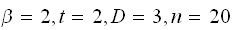
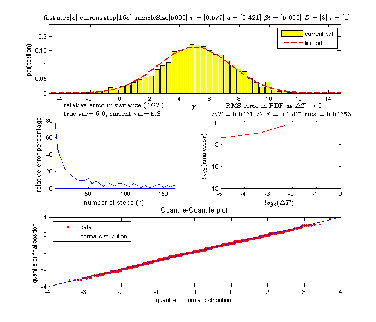
The following diagram below shows a run where on the left side there is a plot
showing the quantile plot when the number of steps is small. The plot on the
right side shows the quantile plot at the end of the run when
 was large. We see that the quantile plot line is now almost exactly over the
 line, confirming that the data is coming from normal distribution.
Therefore, we have answered the 2 questions this simulation was designed to answer.
In doing the above experiments, it was observed that the relative error in the
variance of the final position as
 increased does approach the true variance
 but the convergence is not smooth. As the relative error (around
 to
to
 ),
then increasing
),
then increasing
 more can cause the error to sometimes increase and not decrease as one would
expect. Meaning the relative error is not monotonic decreasing as
more can cause the error to sometimes increase and not decrease as one would
expect. Meaning the relative error is not monotonic decreasing as
 increases. However, as
 becomes very large, the trend is for the relative error is to decrease. I can
only contribute this behavior to some sort of statistical error. This needs to
be investigated more.
becomes very large, the trend is for the relative error is to decrease. I can
only contribute this behavior to some sort of statistical error. This needs to
be investigated more.