By deﬁnition,

∫ ∞ Γ (z ) = tz−1e−tdt 0

Hence

( ) ∫ ∞ Γ n- = t( n2−1)e−tdt 2 0

When $n = 1$ , we are told that

( ) ∫ ∫ 1 ∞ (1−1) −t ∞ (− 1) − t √ -- Γ 2- = t 2 e dt = t 2 e dt = π 0 0

For $n = 3$ , we have

Now do integration by parts,

But $[ 1 ]∞ t2e−t = [0 − 0] = 0 0$ and the above becomes

( ) ∫ ∞ Γ 3- = 1- t(− 12)e− tdt 2 2 0

But $∫ ( ) ∞ t(− 12)e−tdt = Γ 1 0 2$ , hence the above becomes

|------------------| | ( 3) 1 ( 1 ) | Γ -- = --Γ -- | ----2-----2----2----

Now do the same for $n = 5$

But $∫ ∞ (1) −t 0 t 2 e dt$ we found from above to be $(3) Γ 2$ , hence

Γ ( 5) = 3-Γ ( 3-) 2 2 2

But $( ) ( ) Γ 32 = 12Γ 12$ from above, hence

Continuing this way, we ﬁnd that $Γ (7) = 531Γ (1) 2 222 2$ , and hence in general

( n ) (n − 2) (n − 4)(n − 6) 5 31 √-- Γ -- = ------- -------------- ⋅⋅⋅----- π 2 2 2 2 2 22

(1)

Now,

(n − 1)! = (n − 1)(n − 2)(n − 3) (n − 4)(n − 5)(n − 6 )⋅⋅⋅5 × 4 × 3 × 2 × 1

Hence from above we see that

(n − 2 )(n − 4)(n − 6) ⋅⋅⋅5 × 3 × 1 = -------------(n-−-1)!-------------- (n − 1)(n − 3)(n − 5 )⋅⋅⋅4 × 2 × 1

Therefore (1) can be written as

But

( ) (n−21) ( n− 1) − n−21 2n−1- 2 = 2 2 = 2n−21

Hence (2) becomes

( ) (n ) (n − 1)! 1 √ -- Γ -- = --1--------------------------------- ----- π 2 -n−21-(n − 1)(n − 3 )(n − 5)⋅⋅⋅4 × 2 2n−1 2

But there are $n−1- 2$ terms in the expression $(n − 1)(n − 3) (n − 5)⋅⋅⋅4 × 2$ in the denominator above and we have $n− 1 --2-$ number of $1 2$ sitting there, which we can distribute now below each terms to obtain

( ) (n ) (n − 1)! 1 √ -- Γ -- = (n−1)(n−3)(n−5)--------- -n−1- π 2 --2----2----2--⋅⋅⋅ 42 × 22 2

(3)

But

Compare the above to the denominator term in (3) we see it is the same. Hence (3) can be written as

|-(---)-------------------| |Γ n- = (n(-−-1))!--1--√ π| | 2 n−21-! 2n− 1 | ---------------------------

Which is what we are asked to show.

Since $U$ is continuous r.v., we start with the CDF of $Z$

But since $F′U (u) = fU (u )$ , then we know that $∫ b P (a ≤ U ≤ b) = a fU (x)dx → FU (b) − FU (a)$

Hence RHS of (1) becomes

(√ -) ( √ -) FZ (z) = FU z − FU − z

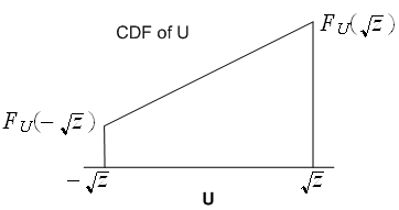
Therefore, taking derivatives with respect to $z$ we obtain

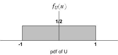
Since $U$ is uniform, hence $fU (a) = fU (− a)$ , hence the above becomes

Now I need to determine the limits of $f (z) Z$ and the shape. $f U$ is deﬁned for real arguments from $− 1$ to $+ 1$ . i.e. $fU$ is real valued function of real arguments. Hence if $z$ was negative then $√ -- z$ will be complex, and so this will not be allowed. Hence we have to restrict $z ≥ 0$ . But now we observe that $z = 0$ is not possible, since we will have $10$ term, so this means $z$ is strictly larger than zero. So

f (z) = √1--f (√z-) z > 0 Z z U

But we know that $f (x) = 1 U 2$ for up to $x = 1$ , hence this means when $√z-> 1$ then $f (√z-) = 0 U$ , when means when $z > 1$ then $√ -- fU ( z) = 0$

Hence we now write

|--------(---------------------------| | || √1--1- 0 < z ≤ 1 | | |{ z 2 | |fZ (z) = 0 z > 1 | | ||| | | ( undef ined z ≤ 0 | -------------------------------------

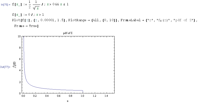
Here is a plot

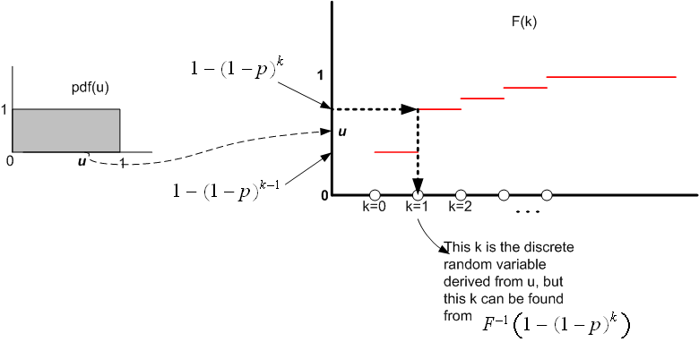
I explain the idea behind obtaining a discrete random number from a continues random number by the following diagram below. We assume that the discrete random number belongs to some distribution. In this example, we are told what the distribution is. We know that the CDF for geometric random variable is given by

F (k) = 1 − (1 − p)k K

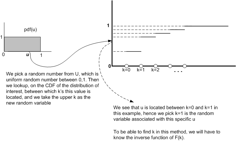
We see from the above diagram, that once we are given $u$ we need to ﬁnd $k$ which satisfy the following identity

FK (k − 1) < u ≤ FK (k)

Or in other words

1 − (1 − p)k− 1 < u ≤ 1 − (1 − p)k

The speciﬁc discrete value $k$ which will satisfy the above, is the random variable we want, which belong to the geometeric distribution.

Now when $u = 0.0153,$ and since $p = 13$ , we have

( 1)k −1 ( 1 )k 1 − 1 − -- < 0.0153 ≤ 1 − 1 − -- 3 3

for $k = 1,$ we have

0 < 0.0153 ≤ 0.33333 YES

Hence $k = 1$ is the random variable associated with $u = 0.0153$

Now let us do $u = 0.7468$

for $k = 1,$ we have

0 < 0.7468 ≤ 0.33333 N O

try $k = 2$

try $k = 3$

try $k = 4$

Hence $k = 4$ is the random variable associated with $u = 0.7468$

Now let us do $u = 0.4451$

We see from the above, that this will have $k = 2$ since for $k = 2$ the intervals is $0.33333 < u ≤ 0.55556$

Hence $k = 2$ is the random variable associated with $u = 0.4451$

Now let us do $u = 0.9318$

From above, we see that this will have a $k$ larger than 4, so we do not need to try from the start, we can start trying from $k = 5$

try $k = 5$

try $k = 6$

try $k = 7$

Hence $k = 7$ is the random variable associated with $u = 0.9318$

Hence result is


$u$	$k$

$0.0153$	$1$

$0.4451$	$2$

$0.7468$	$4$

$0.9318$	$7$

of course one would write a program to do this.

(a)

Let $P (xi = ni)$ means probability of player $i$ winning $ni$ rounds.

We have 3 players, and a total of 10 rounds. Let the players be called $x1,x2,x3$ . Let the number of games WON by $x 1$ be $n 1$ , and number of games won by $x 2$ be $n 2$ , and number of games won by $x 3$ be $n3$ .

Since we have 10 rounds, then we must have 10 wins as well. (some one must win). Hence we have 10 wins and 3 ways to split it, where each 'bucket' is of diﬀerent size. So this is a multi set selection. called multinomial in the book using proposition B in chapter 1, we see that the total number of ways the games can be won is $( ) 10 n1n2n3$

But we need to ﬁnd the probability of each one such combination. So we need to multiply the above by the probability each player wins the number of the games they happened to win, which is $ni P (xi = ni) = p$ , but $1 p = 3$ for each player to win a round. Hence we write

So the above is the joint probability that $p1$ wins $n1$ rounds and $p2$ wins $n2$ rounds and $p3$ wins $n3$ rounds.

(b)We need to ﬁnd $P (x = n ) , 1 1$ i.e. the probability of ﬁrst player winning $n 1$ rounds.

∑ P (x = n ) = P (x = n ,x = n ,x = n ) 1 1 1 1 2 2 3 3 nn23==00,1,1,⋅,⋅⋅⋅⋅⋅1100

To simplify, let me write $P (n1, n2,n3)$ instead, where the position of the $n$ implies the player. So $p (0,1,9)$ means player one wins zero rounds and player 2 wins 1 round and player 3 wins 9 rounds.

So the above becomes

∑ P (x1 = n1) = P (n1,n2,n3) n2=0,1,⋅⋅⋅10 n3=0,1,⋅⋅⋅10

But since $n1 = 10 − (n2 + n3)$ we see that we only need to count those terms in the above sum when this is true. i.e. we do not need to count a term such as $p (1,0,0)$ since this is zero probability of happening. Now we write

P (x1 = n1) = P (n1,10 − n1,0) + P (n1,9 − n1, 1) + P (n1, 8 − n1, 2) + ⋅⋅⋅P (n1, 0,10 − n1)

For example,

$P (x1 = 0) = P (0,10,0) + P (0,9,1) + P (0,8,2) + P (0,7,3) + P (0,6,4) + P (0,5,5) +$

$P (0,4,6) + P (0,3,7) + P (0,2,8) + P (0,1,9) + P (0,0,10)$

But $P (0,10,0 ) = P (0, 0,10)$ and $P (0, 9,1) = P (0,1,9)$ , etc.. so the above can be written as

and

Here is a plot of the marginal probability for player 1 winning $n$ rounds

(a)

Integrate by parts, $dv = e−xdx, u = (x2 − y2)$ , hence $du = 2x$ and $v = − e−x$ , so we obtain

Do integration by parts again, $dv = e− xdx$ , $u = x$ , hence

Hence

|-------------------| |f (y) = 1-(2 − y2)| --Y-------8----------

(b)The hard part is to determine the region to integrate. The following is the needed region which satisfy $P (X + Y ≤ 1)$ and $0 ≤ x ≤ ∞$ and $− x ≤ y ≤ x$

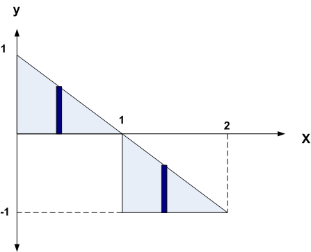
For the top region,

∫ x=1∫ y=1 1-( 2 2) −x I1 = x=0 y=1 −x8 x − y e dydx

and for the bottom region

∫ x=2∫ y= −x 1( ) I2 = --x2 − y2 e−xdydx x=1 y=0 8

Hence

|-----------------∫-----∫----------------------------∫-----∫--------------------------| | x=1 y=1 1 ( 2 2) −x x=2 y=− x1 ( 2 2) −x | |P (X + Y ≤ 1 ) = -- x − y e dydx + -- x − y e dydx | --------------------x=0--y=1−-x8-----------------------x=1--y=0---8--------------------