HW 3.25
Nasser Abbasi
OUTPUT
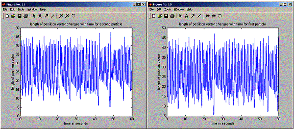
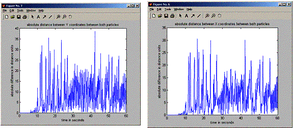
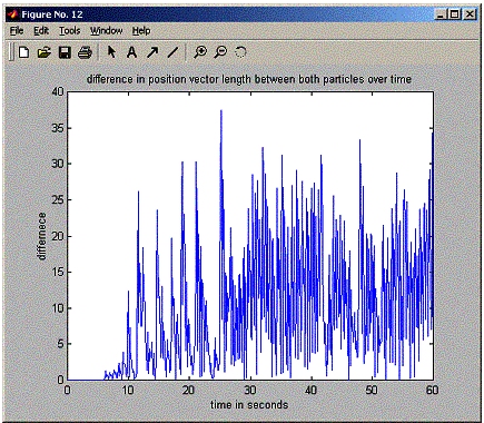
Running this program showed that given a small initial difference in state, at one point in the future, the two trajectories will suddenly diverge from each others over small amount of time, but then the trajectories settle down to distance between them that do not grow much bigger any more as happened the first time, and continue to change by small amount over time. (seen clearly on the log plot below).
» nma_lorenz
nma_lorenz - Program to compute the trajectories of the Lorenz
equations using the non-adaptive Runge-Kutta method.
Nasser Abbasi
HW 3.25
Enter the initial position for the first particle [x y z]: [1 1 20]
Enter the initial position for the second particle [x y z]: [1 1 20.001]
Enter the parameter r: 28
Enter number of steps: 600
Enter time delta tau(sec):0.1
»
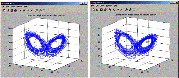
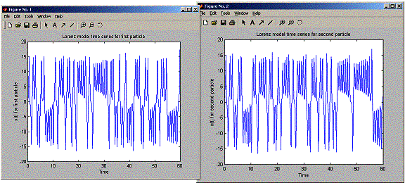
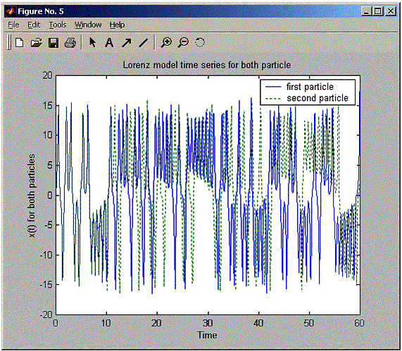
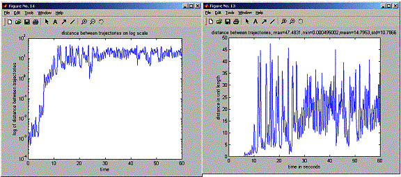
SOURCE CODE
function
nma_lorenz
%
nma_lorenz - Program to compute the trajectories of the Lorenz
%
equations using the non-adaptive Runge-Kutta method.
%
Nasser Abbasi
% HW
3.25
clear; help nma_lorenz;
%
%
layout the data struct used by this program
%
param = struct('r',0,... %this is passed to rk4 or rka
'sigma',0,...
'b',0);
states
= struct( 'state1',[],...
'state2',[]);
positions
= struct('timeVector',[],...
'x1',[],...
'x2',[],...
'y1',[],...
'y2',[],...
'z1',[],...
'z2',[]);
states.state1
= input('Enter the initial position for the first particle [x y z]: ');
states.state2
= input('Enter the initial position for the second particle [x y z]: ');
%
%
get the problem parameter from the user
%
param.r
= input('Enter the parameter r: ');
%
%
These parameters are hardcoded and do not change
%
param.sigma
= 10.;
param.b = 8./3.;
%
%
Obtain the time step and step size, since we are using
%
non adpative rk
%
currentTime = 0;
numberOfSteps
= input('Enter number of steps: ');
tau = input('Enter time delta
tau(sec):');
%
%
All, set, lets start the simulation
%
for
i=1:numberOfSteps
positions = recordStateInstance(i,states,positions,currentTime);
%
% Apply non-adaptive rk to both particles at
the time time.
%
states.state1 =
rk4(states.state1,currentTime,tau,'lorzrk',param);
states.state2 =
rk4(states.state2,currentTime,tau,'lorzrk',param);
currentTime = currentTime + tau;
end
%
%
End of simulation, lets analyse the output, and do the plots
%
(the fun part)
%
analyseAndPlot(positions,param);
return;
%%%%%%%%%%%%%%%%%%%%%%%%%%%%%%%%%%%%%%%%%%%%%
%
Saves the state at each time step for later analysis
%
and plotting when the simulation is completed.
%
%%%%%%%%%%%%%%%%%%%%%%%%%%%%%%%%%%%%%%%%%%%%%%%
function positions =
recordStateInstance(stepNumber,states,positions,time)
positions.x1(stepNumber) = states.state1(1);
positions.y1(stepNumber) = states.state1(2);
positions.z1(stepNumber) = states.state1(3);
positions.x2(stepNumber) = states.state2(1);
positions.y2(stepNumber) = states.state2(2);
positions.z2(stepNumber) = states.state2(3);
% record the time elapsed since start of
simulation at this step number
% we could ofcourse find this by
stepNumber*tau, since this is non adaptive
% R-K, but this might be usefull to keep in
this form for some kinds of
% plotting later on.
positions.timeVector(stepNumber) = time;
return;
%%%%%%%%%%%%%%%%%%%%%%%%%%%%%%%%%%%%%%%%%%%%%%
%
function to analys and plot the result of the
%
simulation. Takes as input the positions history of
%
the two particles and determines the change in
%
trajectories over time.
%%%%%%%%%%%%%%%%%%%%%%%%%%%%%%%%%%%%%%%%%%%%%%%
function
analyseAndPlot(positions,param)
%
%
First, lets plot time series for X position for each particle
%
figure;
plot(positions.timeVector,
positions.x1,'-')
xlabel('Time'); ylabel('x(t) for first particle')
title(sprintf('Lorenz
model time series for first particle'));
figure;
plot(positions.timeVector,
positions.x2,'-')
xlabel('Time'); ylabel('x(t) for second particle')
title(sprintf('Lorenz
model time series for second particle'));
%
%
Graph the x,y,z phase space trajectory for both particles
%
%
Mark the location of the three steady states
x_ss(1)
= 0;
y_ss(1)
= 0;
z_ss(1)
= 0;
x_ss(2)
= sqrt(param.b*(param.r-1));
y_ss(2)
= x_ss(2);
z_ss(2)
= param.r-1;
x_ss(3)
= -sqrt(param.b*(param.r-1));
y_ss(3)
= x_ss(3);
z_ss(3)
= param.r-1;
figure;
plot3(positions.x1,positions.y1,positions.z1,'-',x_ss,y_ss,z_ss,'*')
view([30
20]); % Rotate to get a better view
grid; % Add a grid to aid perspective
xlabel('x');
ylabel('y'); zlabel('z');
title('Lorenz
model phase space for first particle');
figure;
plot3(positions.x2,positions.y2,positions.z2,'-',x_ss,y_ss,z_ss,'*')
view([30
20]); % Rotate to get a better view
grid; % Add a grid to aid perspective
xlabel('x');
ylabel('y'); zlabel('z');
title('Lorenz
model phase space for second particle');
%
%
Now, let me plot the time series for X for both particles on the
%
the same plot
%
figure;
plot(positions.timeVector,
positions.x1,'-',positions.timeVector,positions.x2,':')
xlabel('Time'); ylabel('x(t) for both particles')
title(sprintf('Lorenz
model time series for both particle'));
legend('first
particle','second particle');
%
%
Now find the distance between the particles in each dimension and
%
plot
%
figure;
plot(positions.timeVector,
abs(positions.x1-positions.x2),'-');
title('absolute
distance between X coordinates between both particles');
xlabel('time
in seconds');
ylabel('absolute
difference in distance units');
%
%
Now find the distance between the particles in each dimension and
%
first, I plot distance between each coordinate
%
figure;
plot(positions.timeVector,
abs(positions.y1-positions.y2),'-');
title('absolute
distance between Y coordinates between both particles');
xlabel('time
in seconds');
ylabel('absolute
difference in distance units');
%
%
Now find the distance between the particles in each dimension and
%
plot
%
figure;
plot(positions.timeVector,
abs(positions.z2-positions.z2),'-');
title('absolute
distance between z coordinates between both particles');
xlabel('time
in seconds');
ylabel('absolute
difference in distance units');
%
%
plot the difference between the length of the position vector
%
%
figure;
for(i=1:length(positions.timeVector))
r1(i)= sqrt(positions.x1(i)^2 +
positions.y1(i)^2 + positions.z1(i)^2 );
r2(i)= sqrt(positions.x2(i)^2 +
positions.y2(i)^2 + positions.z2(i)^2 );
distanceTraj(i) = sqrt( (positions.x1(i)-positions.x2(i))^2 + ...
(positions.y1(i)-positions.y2(i))^2 + ...
(positions.z1(i)-positions.z2(i))^2 );
end
figure;
plot(positions.timeVector,r1,'-');
title('length
of posiition vector changes with time for first particle');
xlabel('time
in seconds');
ylabel('length
of position vector');
figure;
plot(positions.timeVector,r2,'-');
title('length
of posiition vector changes with time for second particle');
xlabel('time
in seconds');
ylabel('length
of position vector');
figure;
plot(positions.timeVector,abs(r1-r2),'-');
title('difference
in position vector length between both particles over time');
xlabel('time
in seconds');
ylabel('differnece');
%
%
Now, plot the distance between the trajectoris
%
figure;
plot(positions.timeVector,distanceTraj,'-');
title(sprintf('distance
between trajectories, max=%g,min=%g,mean=%g,std=%g',...
max(distanceTraj),min(distanceTraj),mean(distanceTraj),std(distanceTraj)));
xlabel('time
in seconds');
ylabel('distance
in unit length');
figure;
semilogy(positions.timeVector,distanceTraj);
title('distance
between trajectories on log scale');
xlabel('time');
ylabel('log
of distance between trajectories');
function
deriv = lorzrk(s,t,param)
% Returns right-hand side of Lorenz model ODEs
% Inputs
% s
State vector [x y z]
% t
Time (not used)
% param
Parameters [r sigma b]
% Output
% deriv
Derivatives [dx/dt dy/dt dz/dt]
%*
For clarity, unravel input vectors
x = s(1);
y = s(2);
z = s(3);
r = param.r;
sigma
= param.sigma;
b = param.b;
%*
Return the derivatives [dx/dt dy/dt dz/dt]
deriv(1)
= sigma*(y-x);
deriv(2)
= r*x - y - x*z;
deriv(3)
= x*y - b*z;
return;