HW 3.23

Nasser Abbasi

OUTPUT

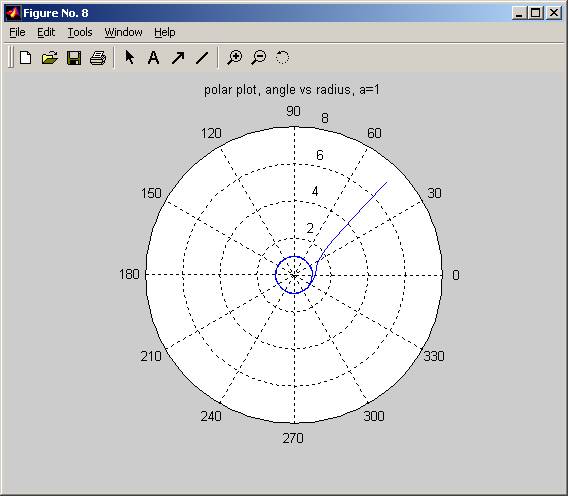
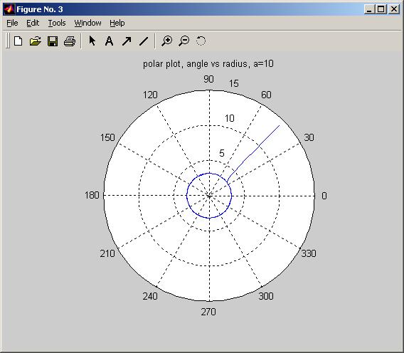
The first two runs for a>0, they show that particle spirles to around a circle of radius sqrt(a).

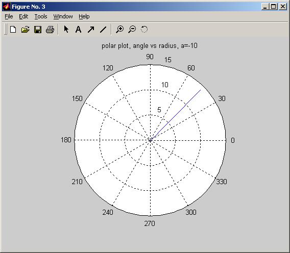
The third plot for a<0, it shows the particle spirles to the origin.

» nma_HW_3_23

nma_HW_3_23 - Program to solve HW 3.23

Enter x initial value (m): 5

Enter y initial value (m): 5

Enter number of steps: 100

Enter time step (sec): 0.1

parameter a value:1

Final radius is 0.999951

a=1, sqrt(a)=1

»

» nma_HW_3_23

nma_HW_3_23 - Program to solve HW 3.23

Enter x initial value (m): 10

Enter y initial value (m): 10

Enter number of steps: 200

Enter time step (sec): 0.1

parameter a value:10

Final radius is 3.16218

a=10, sqrt(a)=3.16228

» nma_HW_3_23

nma_HW_3_23 - Program to solve HW 3.23

Enter x initial value (m): 10

Enter y initial value (m): 10

Enter number of steps: 200

Enter time step (sec): 0.1

parameter a value:-10

Final radius is 1.20127e-018

a=-10, sqrt(a)=0

»

SOURCE CODE

% nma_HW_3_23 - Program to solve HW 3.23

clear all; help nma_HW_3_23; % Clear memory and print header

%

% Nasser Abbasi, HW 3.23

%

%* Set initial position of the particle.

x0 = input('Enter x initial value (m): ');

y0 = input('Enter y initial value (m): ');

x_now = x0;

y_now = y0;

state = [ x_now y_now ]; % Used by R-K routines

%

% Parameter to pass to the R-K integrator via rk4.

%

param = struct( 'a',0 );

% set rk adaptive error, and initialize time

adaptErr = 1.e-3; % Error parameter used by adaptive Runge-Kutta

time = 0;

%* Loop over desired number of steps using specified

% numerical method.

nStep = input('Enter number of steps: ');

tau = input('Enter time step (sec): ');

a = input('parameter a value:');

param.a=a;

for iStep=1:nStep

%* Record position and energy for plotting.

xplot(iStep) = x_now; % Record position for polar plot

yplot(iStep) = y_now;

tplot(iStep) = time;

[state time tau] = rka(state,time,tau,adaptErr,'nma_HW_3_23_deriv',param);

x_now = [state(1)]; % 4th order Runge-Kutta

y_now = [state(2)];

end

for(i=1:length(tplot))

radius(i) = sqrt(xplot(i)^2+yplot(i)^2);

angle(i) = atan2(yplot(i),xplot(i));

end

fprintf('Final radius is %g\n',radius(end));

fprintf('a=%g, sqrt(a)=%g\n',a,sqrt(a));

figure;

plot(xplot,yplot);

title(sprintf('X vs Y plot, a=%g',a));

xlabel('X in meter');

ylabel('Y in meter');

figure;

polar(xplot);

title('x in polar plot');

figure;

polar(angle,radius);

title(sprintf('polar plot, angle vs radius, a=%g',a));

function deriv = nma_HW_3_23_deriv(s,t,param)

% Returns right-hand side of HW 2.3; used by Runge-Kutta routines

% problem 3.23

%

% Inputs

% s State vector [x y]

% t not used

% param Parameter struct

% Output

% deriv Derivatives

% Nasser Abbasi, feb 25. 2002.

x= s(1);

y= s(2);

a= param.a;

deriv(1) = a*x+y-x*(x^2+y^2);

deriv(2) = -x+a*y-y*(x^2+y^2);

return;