HW 3.14

Nasser Abbasi

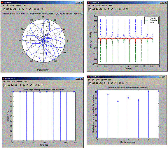
Output

» nma_orbit

nma_orbit - Program to compute the orbit of a comet.

Enter initial radial distance (AU): 1

Enter initial tangential velocity (AU/yr): pi/2

Enter alpha constant for the problem:0.02

Enter number of steps: 300

Enter time step (yr): 0.005

Max r occured at time step=1, norm(r)=1 AU, angle=0 degree

formula says -46.6602 degree

Max r occured at time step=34, norm(r)=0.998302 AU, angle=-47.6152 degree

formula says -44.488 degree

Max r occured at time step=65, norm(r)=0.994744 AU, angle=-91.8046 degree

formula says -41.6312 degree

Max r occured at time step=99, norm(r)=0.999155 AU, angle=-140.422 degree

formula says -46.1857 degree

Max r occured at time step=130, norm(r)=0.99318 AU, angle=175.068 degree

formula says -40.4269 degree

Max r occured at time step=163, norm(r)=0.99966 AU, angle=126.568 degree

formula says -46.6301 degree

Max r occured at time step=194, norm(r)=0.999733 AU, angle=80.069 degree

formula says -46.6631 degree

Max r occured at time step=228, norm(r)=0.996806 AU, angle=32.1933 degree

formula says -43.5446 degree

Max r occured at time step=258, norm(r)=0.98758 AU, angle=-15.6186 degree

formula says -36.5409 degree

Max r occured at time step=293, norm(r)=0.999583 AU, angle=-59.831 degree

formula says -46.6148 degree

SOURCE CODE

% nma_orbit - Program to compute the orbit of a comet.

clear all; help nma_orbit; % Clear memory and print header

%

% Nasser Abbasi, HW 3.14 Modified from teacher orbit.m

%

%* Set initial position and velocity of the comet.

r0 = input('Enter initial radial distance (AU): ');

v0 = input('Enter initial tangential velocity (AU/yr): ');

r_now = [r0 0];

v_now = [0 v0];

%

% Save initial angle, since I'll need this to find

% the number of time steps it takes to cycle back to it.

% which tells me how long one revolution it

%

initialAngleInRadian = atan2(r_now(2),r_now(1));

alpha = input('Enter alpha constant for the problem:');

state = [ r_now(1) r_now(2) v_now(1) v_now(2) ]; % Used by R-K routines

%

% Parameter to pass to the R-K integrator via rk4.

%

param = struct( 'alpha',0, ...

'GM',0);

%* Set physical parameters (mass, G*M)

param.GM = 4*pi^2; % Grav. const. * Mass of Sun (au^3/yr^2)

param.alpha = alpha; % constant for the force factor, see problem description.

mass = 1.; % Mass of comet

adaptErr = 1.e-3; % Error parameter used by adaptive Runge-Kutta

time = 0;

%* Loop over desired number of steps using specified

% numerical method.

nStep = input('Enter number of steps: ');

tau = input('Enter time step (yr): ');

numberOfSignChanges = 0;

lastAngle = initialAngleInRadian;

revolutionNumber = 0;

numberOfStepsLastRevolution = 0;

iStepUpToLastRevolution = 0;

for iStep=1:nStep

%timeValue(iStep)= time;

%* Record position and energy for plotting.

rplot(iStep) = norm(r_now); % Record position for polar plot

thplot(iStep) = atan2(r_now(2),r_now(1));

%

% L, the anguler momentum is tracked.

L(iStep) = norm(r_now) * norm(v_now);

%

% This is extra, I keep track of how many time steps it

% takes to make one revolution to plot at the end.

%

if( thplot(iStep) * lastAngle < 0 )

numberOfSignChanges = numberOfSignChanges + 1;

if( numberOfSignChanges == 2 )

revolutionNumber = revolutionNumber + 1;

numberOfStepsLastRevolution = iStep - iStepUpToLastRevolution;

iStepUpToLastRevolution = iStep;

numberOfStepsPerRevolution( revolutionNumber ) = numberOfStepsLastRevolution;

numberOfSignChanges = 0;

end;

end;

lastAngle = thplot(iStep);

tplot(iStep) = time;

kinetic(iStep) = .5*mass*norm(v_now)^2; % Record energies

potential(iStep) = - param.GM*mass/norm(r_now);

[state time tau] = rka(state,time,tau,adaptErr,'nma_HW_3_14_deriv',param);

r_now = [state(1) state(2)]; % 4th order Runge-Kutta

v_now = [state(3) state(4)];

end

%

% ignore the first revolution, since it could have started anywhere, then look

% for 2 complete revlutions, and use always revolution 2 and 3 to find the

% precesses angle

%

if( revolutionNumber < 3 )

fprintf('Please run the simulation for longer time, need at least 2 complete revolutions!');

return;

end

%

% extra: I have at least 2 revolutions, plot time it takes to make one

% revolution. We will see each revolution is taking less time to compelte

% than the last one

%

figure;

stem(numberOfStepsPerRevolution);

title('number of time steps to complete one revolution');

xlabel('Revolution number');

ylabel('Number time steps to complete the revolution');

Axis([1 revolutionNumber 0 max(numberOfStepsPerRevolution)]);

%

% find the all the indexes where max norm(r) occured

% I need to do this, since this tells me the angles needed

%

j=0;

i=1;

maxRecorded=0;

while(1)

i=i+1;

if( i > length(rplot))

break;

end

if(rplot(i) < rplot(i-1))

if( ~maxRecorded)

j=j+1;

maxNorm(j,1) = rplot(i-1); %column 1 has the norm

maxNorm(j,2) = i-1; %column 2 has the index

maxRecorded =1;

end

else

maxRecorded =0;

end

end

%

% Plot the time steps at which max norm(r) occured

%

figure;

stem(maxNorm(:,2),maxNorm(:,1));

title('Time steps where position vector was maximum');

xlabel('Time step');

ylabel('Norm(r) in AU');

for(i=1:length(maxNorm))

angleInDegree= thplot(maxNorm(i,2)) * 180 / pi;

fprintf('Max r occured at time step=%d, norm(r)=%g AU, angle=%g degree\n', ...

maxNorm(i,2),maxNorm(i,1), angleInDegree );

a = sqrt( 1 + ((param.GM * param.alpha)/ L(maxNorm(i,2))^2) );

formulaPrecess= 360*(1-a)/a;

fprintf('formula says %g degree\n',formulaPrecess);

end

%* Graph the trajectory of the comet.

figure;

polar(thplot,rplot,'-'); % Use polar plot for graphing orbit

xlabel('Distance (AU)'); grid;

S=sprintf('Initial radial=%g (AU), Initial V=%g (AU/yr), tau=%g (AU yr), nStep=%d, Alpha=%g',r0,v0,tau,nStep,alpha);

title(S);

pause(1) % Pause for 1 second before drawing next plot

%* Graph the energy of the comet versus time.

figure;

totalE = kinetic + potential; % Total energy

plot(tplot,kinetic,'-.',tplot,potential,'--',tplot,totalE,'-')

legend('Kinetic','Potential','Total');

xlabel('Time (yr)'); ylabel('Energy (M AU^2/yr^2)');

function deriv = nma_HW_3_14_deriv(s,t,param)

% Returns right-hand side of Kepler ODE; used by Runge-Kutta routines

% Moified for problem 3.14

%

% Inputs

% s State vector [r(1) r(2) v(1) v(2)]

% t Time (not used)

% param Parameter struct

% Output

% deriv Derivatives [dr(1)/dt dr(2)/dt dv(1)/dt dv(2)/dt]

% Nasser Abbasi, feb 19. 2002.

%* Compute acceleration

r = [s(1) s(2)]; % Unravel the vector s into position and velocity

v = [s(3) s(4)];

accel = - param.GM*r/norm(r)^3; % Gravitational acceleration

accel = accel * (1 - (param.alpha/norm(r)) );

%* Return derivatives [dr(1)/dt dr(2)/dt dv(1)/dt dv(2)/dt]

deriv = [v(1) v(2) accel(1) accel(2)];

return;