HW 3, problem 1.16. PHY 240
By Nasser Abbasi.
Source code
File nma_interp.m
%nma_interp - Program to
interpolate data using Lagrange
%polynomial to fit a polynimal to
any number of points
%HW 3, 1.16, by Nasser Abbasi, San
Jose State Univ.
%PHY 240. Feb 2, 2002.
% design notes:
% We use the general form of
lagrange interpolation for
% any points
%
% (X-X2)(X-X3)...(X-Xn)
% P(x) =
------------------------- Y1
% (X1-X2)(X1-X3)...(X1-Xn)
% +
% (X-X1)(X-X3)...(X-Xn)
% -------------------------
Y2
% (X2-X1)(X2-X3)...(X2-Xn)
% + .....
%
% (X-X1)(X-X1)...(X-Xn-1)
% -------------------------
Yn
% (Xn-X2)(Xn-X3)...(Xn-Xn-1)
%
%
clear all; help nma_interp;
%* Initialize the data points to
be fit by quadratic
disp('Enter data
points as x,y paris (e.g., [1 2], when done, enter RETURN with empty line');
pointNumber = 0;
point = input('Enter
data point:');
while ~isempty(point)
pointNumber = pointNumber +1;
X(
pointNumber ) = point(1);
Y(
pointNumber ) = point(2);
point =
input('Enter data point:');
end
if pointNumber == 0
disp('You entered no points, please try again');
return;
end
% Tell the user the points they
entered before proceeding
disp('You entered
these points:');
for i=1:pointNumber
disp(sprintf('Point %d = [%g %g]',i,X(i),Y(i)));
end
%* Establish the range of
interpolation (from x_min to x_max)
xr = input('Enter
range of x values as [x_min xmax]: ');
%* find yi for the desired
interpolation values xi using
%
the function intrpf
disp(sprintf('Interpolating
polynomial is\nX\tY\t'));
nplot = 100;
%Number of points for interpolation
curve
for i=1:nplot
xi(i) =
xr(1) + ( xr(2)-xr(1))*(i-1)/(nplot-1);
yi(i) =
nma_interpf(xi(i),X,Y); % Use interpf function to interpolate
% print the X,Y values of the interpolation polynmial
to check if
% correct by comparing to tables
disp(sprintf('%g\t%g',xi(i),yi(i)));
end
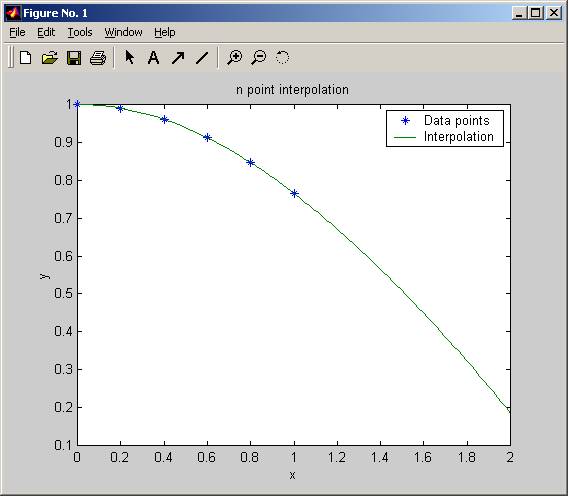
%* Plot the curve given by (xi,yi)
and mark original data points
plot(X,Y,'*',xi,yi,'-');
xlabel('x');
ylabel('y');
title('n point
interpolation');
legend('Data points','Interpolation');
File nma_interpf.m
function yi = nma_interpf(xi,X,Y)
% Function to interpolate between
data points
% using Lagrange polynomial
% Inputs
% X Vector of x
coordinates of data points
% Y Vector of y
coordinates of data points
% xi The x value where interpolation is computed
% Output
% yi The interpolation polynomial evaluated at xi
% by Nasser Abbasi, HW3, PYS 240
% feb 2, 2002.
% Use the general form of lagrange
interpolation for
% any points
%
% (X-X2)(X-X3)...(X-Xn)
% P(x) =
------------------------- Y1
% (X1-X2)(X1-X3)...(X1-Xn)
% +
% (X-X1)(X-X3)...(X-Xn)
% -------------------------
Y2
% (X2-X1)(X2-X3)...(X2-Xn)
% + .....
%
% (X-X1)(X-X1)...(X-Xn-1)
% -------------------------
Yn
% (Xn-X2)(Xn-X3)...(Xn-Xn-1)
% Calculate yi = p(xi) using
Lagrange polynomial
numberOfPoints = length(X);
yi=0;
for i=1:numberOfPoints
% Initialize numerator and denomiator each term
term
numerator=1;
denominator=1;
for j=1:numberOfPoints
if( i ~= j )
numerator = numerator
* (xi-X(j));
denominator = denominator *
(X(i)-X(j));
end
end
yi = yi +
( (numerator/denominator)*Y(i) );
end
RESULTS and OUTPUT
» nma_interp
nma_interp - Program to interpolate data using Lagrange
polynomial to fit a polynimal to any number of points
Enter data points as x,y paris (e.g., [1 2], when done, enter RETURN with empty line
Enter data point: [0 1]
Enter data point: [0.2 0.99]
Enter data point: [0.4 0.9604]
Enter data point: [0.6 0.912]
Enter data point: [0.8 0.8463]
Enter data point: [1.0 0.7652]
Enter data point:
You entered these points:
Point 1 = [0 1]
Point 2 = [0.2 0.99]
Point 3 = [0.4 0.9604]
Point 4 = [0.6 0.912]
Point 5 = [0.8 0.8463]
Point 6 = [1 0.7652]
Enter range of x values as [x_min xmax]: [0 2]
Interpolating polynomial is
X Y
0 1
0.020202 0.999883
0.040404 0.999567
0.0606061 0.99905
0.0808081 0.998333
0.10101 0.997414
0.121212 0.996294
0.141414 0.994972
0.161616 0.993449
0.181818 0.991724
0.20202 0.989798
0.222222 0.987672
0.242424 0.985345
0.262626 0.982819
0.282828 0.980093
0.30303 0.977169
0.323232 0.974047
0.343434 0.970729
0.363636 0.967215
0.383838 0.963506
0.40404 0.959604
0.424242 0.95551
0.444444 0.951225
0.464646 0.946751
0.484848 0.942088
0.505051 0.93724
0.525253 0.932206
0.545455 0.926989
0.565657 0.92159
0.585859 0.916011
0.606061 0.910254
0.626263 0.904321
0.646465 0.898214
0.666667 0.891934
0.686869 0.885483
0.707071 0.878864
0.727273 0.872078
0.747475 0.865127
0.767677 0.858014
0.787879 0.85074
0.808081 0.843308
0.828283 0.83572
0.848485 0.827977
0.868687 0.820082
0.888889 0.812037
0.909091 0.803844
0.929293 0.795505
0.949495 0.787022
0.969697 0.778398
0.989899 0.769634
1.0101 0.760732
1.0303 0.751695
1.05051 0.742524
1.07071 0.733222
1.09091 0.72379
1.11111 0.714231
1.13131 0.704546
1.15152 0.694737
1.17172 0.684805
1.19192 0.674754
1.21212 0.664584
1.23232 0.654297
1.25253 0.643894
1.27273 0.633378
1.29293 0.62275
1.31313 0.61201
1.33333 0.601162
1.35354 0.590205
1.37374 0.579141
1.39394 0.567971
1.41414 0.556697
1.43434 0.545319
1.45455 0.533838
1.47475 0.522255
1.49495 0.510571
1.51515 0.498786
1.53535 0.486901
1.55556 0.474916
1.57576 0.462832
1.59596 0.450649
1.61616 0.438366
1.63636 0.425985
1.65657 0.413504
1.67677 0.400924
1.69697 0.388244
1.71717 0.375464
1.73737 0.362582
1.75758 0.349599
1.77778 0.336514
1.79798 0.323325
1.81818 0.310031
1.83838 0.296631
1.85859 0.283123
1.87879 0.269506
1.89899 0.255778
1.91919 0.241937
1.93939 0.227981
1.9596 0.213908
1.9798 0.199715
2 0.1854
»
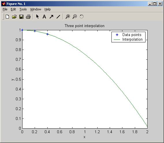
Now, Run teach_interp (original text book) and see if result has improved
» teach_interp
teach_interp - Program to interpolate data using Lagrange
polynomial to fit quadratic to three data points
Enter data points as x,y paris (e.g., [1 2]
Enter data point:[0 1.0]
Enter data point:[0.2 0.9900]
Enter data point:[0.4 0.9604]
Enter range of x values as [x_min xmax]: [0 2]
»
To find is estimate improved, I need to modify teach_interp to make it print the values of the interpolating polynomial so I can compare.
So, I did that and rerun the above.
» teach_interp
teach_interp - Program to interpolate data using Lagrange
polynomial to fit quadratic to three data points
Enter data points as x,y paris (e.g., [1 2]
Enter data point:[0 1.0]
Enter data point:[0.2 0.9900]
Enter data point:[0.4 0.9604]
Enter range of x values as [x_min xmax]: [0 2]
0 1
0.020202 0.99988
0.040404 0.99956
0.0606061 0.999039
0.0808081 0.998319
0.10101 0.997399
0.121212 0.996279
0.141414 0.994959
0.161616 0.993439
0.181818 0.991719
0.20202 0.989799
0.222222 0.987679
0.242424 0.985359
0.262626 0.982839
0.282828 0.980119
0.30303 0.977199
0.323232 0.974079
0.343434 0.97076
0.363636 0.96724
0.383838 0.96352
0.40404 0.9596
0.424242 0.95548
0.444444 0.95116
0.464646 0.946641
0.484848 0.941921
0.505051 0.937001
0.525253 0.931882
0.545455 0.926562
0.565657 0.921042
0.585859 0.915323
0.606061 0.909403
0.626263 0.903284
0.646465 0.896964
0.666667 0.890444
0.686869 0.883725
0.707071 0.876805
0.727273 0.869686
0.747475 0.862366
0.767677 0.854847
0.787879 0.847128
0.808081 0.839208
0.828283 0.831089
0.848485 0.82277
0.868687 0.81425
0.888889 0.805531
0.909091 0.796612
0.929293 0.787492
0.949495 0.778173
0.969697 0.768654
0.989899 0.758935
1.0101 0.749015
1.0303 0.738896
1.05051 0.728577
1.07071 0.718058
1.09091 0.707339
1.11111 0.69642
1.13131 0.685301
1.15152 0.673982
1.17172 0.662463
1.19192 0.650744
1.21212 0.638825
1.23232 0.626706
1.25253 0.614387
1.27273 0.601868
1.29293 0.589149
1.31313 0.57623
1.33333 0.563111
1.35354 0.549792
1.37374 0.536273
1.39394 0.522555
1.41414 0.508636
1.43434 0.494517
1.45455 0.480198
1.47475 0.46568
1.49495 0.450961
1.51515 0.436042
1.53535 0.420924
1.55556 0.405605
1.57576 0.390086
1.59596 0.374368
1.61616 0.358449
1.63636 0.342331
1.65657 0.326012
1.67677 0.309494
1.69697 0.292775
1.71717 0.275857
1.73737 0.258738
1.75758 0.24142
1.77778 0.223901
1.79798 0.206183
1.81818 0.188264
1.83838 0.170146
1.85859 0.151828
1.87879 0.133309
1.89899 0.114591
1.91919 0.0956729
1.93939 0.0765546
1.9596 0.0572364
1.9798 0.0377182
2 0.018
»
Results
|
X |
Theortical Y (from table) |
Y (from 3 points interp) |
Y (from 6 points interp) |
difference |
|
0 |
1 |
1 |
1 |
0 |
|
0.2 |
0.990024972239576 |
0.989799 |
0.989798 |
0.000001 |
|
0.4 |
0.960398226659563 |
0.959600 |
0.959604 |
0.000004 |
Using 6 points interpolation has improved the result slightly.