Problem 7.5

Nasser Abbasi

Output

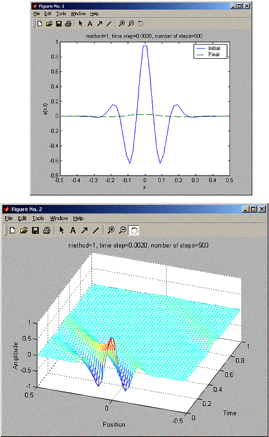
Changed the advect program to use the upwind schem. Run the program to generate the plots shown in figure 7.3, 7.4, 7.5, 7.6 and 7.7

Conclusion

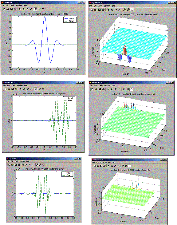
For the FTCS method, the signal at the end almost died out, no amplitude at the final time. Tried for tau=0.002

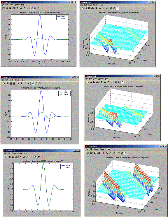
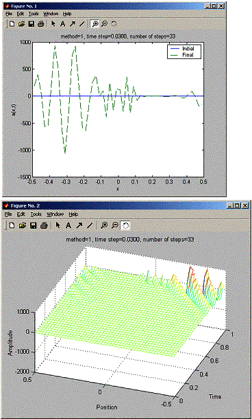
To see the effect of increasing time step on the FTCS method using the upwind scheme I rerun the program with tau=0.01, 0.015 and 0.02. This shows as Tau increased to 0.02 (h/c), The final wave become closer to the initial wave. Next I tried FTCS for tau=0.03, then I see it became not stable. So for tau > tw, FTCS is not stable using the upwind scheme.

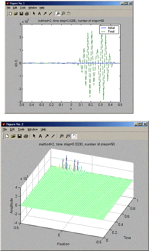
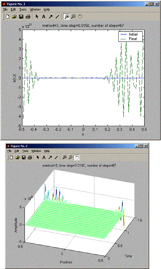
Next, I run LAX for tau=0.0001, 0.02 and 0.03. This show Lax not stable , even for tau=0.02. Also the same problem showed for LAX-wendroff (this makes me worried I made a mistake somewhere?)

» nma_advect_problem_7_5

nma_advect_problem_7_5 - Program to solve the

advection equation using the various hyperbolic PDE schemes

solves problem 7.5 in book, modified from book advect.m

Nasser Abbasi

select numerical method: FTCS=1, Lax=2 Lax-Wendroff=3 :1

You selected method 1

Enter number of grid points: 50

Time for wave to move one grid spacing is 0.02

Enter time step: 0.002

Wave circles system in 500 steps

Enter number of steps: 500

»

To see the effect of increasing time step on the FTCS method using the upwind scheme I rerun the program with tau=0.01, 0.015 and 0.02. This shows as Tau increased to 0.02 (h/c), The final wave become closer to the initial wave.

» nma_advect_problem_7_5

select numerical method: FTCS=1, Lax=2 Lax-Wendroff=3 :1

You selected method 1

Enter number of grid points: 50

Time for wave to move one grid spacing is 0.02

Enter time step: 0.03

Wave circles system in 33.3333 steps

Enter number of steps: 33

» nma_advect_problem_7_5

nma_advect_problem_7_5 - Program to solve the

advection equation using the various hyperbolic PDE schemes

solves problem 7.5 in book, modified from book advect.m

Nasser Abbasi

select numerical method: FTCS=1, Lax=2 Lax-Wendroff=3 :2

You selected method 2

Enter number of grid points: 50

Time for wave to move one grid spacing is 0.02

Enter time step: 0.02

Wave circles system in 50 steps

Enter number of steps: 50

»

» nma_advect_problem_7_5

nma_advect_problem_7_5 - Program to solve the

advection equation using the various hyperbolic PDE schemes

solves problem 7.5 in book, modified from book advect.m

Nasser Abbasi

select numerical method: FTCS=1, Lax=2 Lax-Wendroff=3 :2

You selected method 2

Enter number of grid points: 50

Time for wave to move one grid spacing is 0.02

Enter time step: 0.015

Wave circles system in 66.6667 steps

Enter number of steps: 67

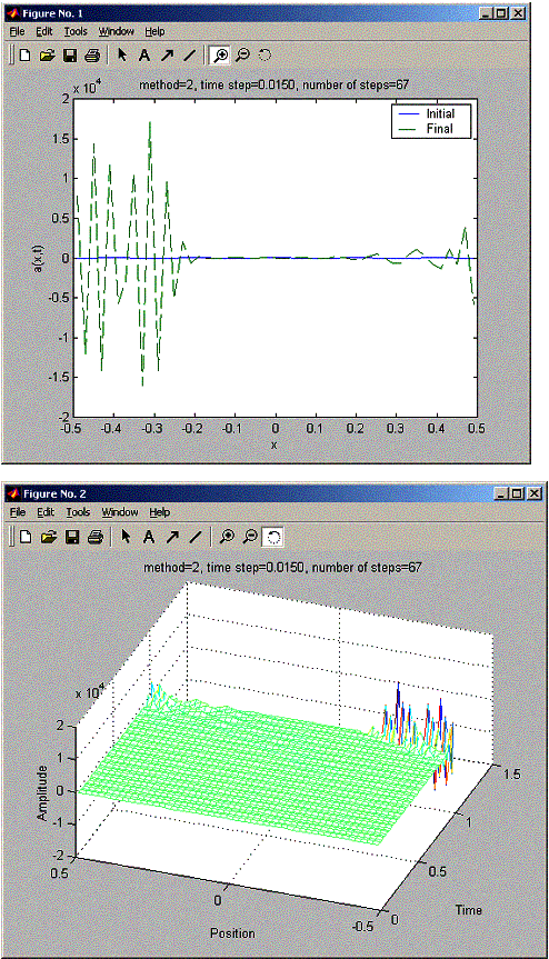
Next, I run LAX for tau=0.0001, 0.02 and 0.03. This show Lax not stable .

» nma_advect_problem_7_5

nma_advect_problem_7_5 - Program to solve the

advection equation using the various hyperbolic PDE schemes

solves problem 7.5 in book, modified from book advect.m

Nasser Abbasi

select numerical method: FTCS=1, Lax=2 Lax-Wendroff=3 :3

You selected method 3

Enter number of grid points: 50

Time for wave to move one grid spacing is 0.02

Enter time step: 0.015

Wave circles system in 66.6667 steps

Enter number of steps: 67

SOURCE

function nma_advect_problem_7_5()

% nma_advect_problem_7_5 - Program to solve the

% advection equation using the various hyperbolic PDE schemes

% solves problem 7.5 in book, modified from book advect.m

% Nasser Abbasi

clear all; help nma_advect_problem_7_5; % Clear memory and print header

%* Select numerical parameters (time step, grid spacing, etc.).

try_again=1;

while(try_again)

method = input('select numerical method: FTCS=1, Lax=2 Lax-Wendroff=3 :');

if( method<1 | method>3 )

fprintf('Please try again, choice must be 1 or 2 or 3.\n');

else

try_again=0;

fprintf('You selected method %d\n',method);

end

end

N = input('Enter number of grid points: ');

L = 1.; % System size

h = L/N; % Grid spacing

c = 1; % Wave speed

fprintf('Time for wave to move one grid spacing is %g\n',h/c);

tau = input('Enter time step: ');

%coeff = -c*tau/(2.*h); % Coefficient used by all schemes

%

% change coeff for the 'upwind' scheme

%

coeff = -c*tau/(h); % Coefficient used by all schemes

coefflw = 2*coeff^2; % Coefficient used by L-W scheme

fprintf('Wave circles system in %g steps\n',L/(c*tau));

nStep = input('Enter number of steps: ');

%* Set initial and boundary conditions.

sigma = 0.1; % Width of the Gaussian pulse

k_wave = pi/sigma; % Wave number of the cosine

x = ((1:N)-1/2)*h - L/2; % Coordinates of grid points

% Initial condition is a Gaussian-cosine pulse

a = cos(k_wave*x) .* exp(-x.^2/(2*sigma^2));

% Use periodic boundary conditions

%ip(1:(N-1)) = 2:N; ip(N) = 1; % ip = i+1 with periodic b.c.

%im(2:N) = 1:(N-1); im(1) = N; % im = i-1 with periodic b.c.

%

% changed the boundary conditions since now we have

% a(i)-a(i-1) instead of a(i+1)-a(i-1). in this, ip is the

% the left term and im is the right term.

%

ip(1:N) = 1:N;

im(2:N) = 1:(N-1);

im(1) = N; % im = i-1 with periodic b.c.

%* Initialize plotting variables.

iplot = 1; % Plot counter

aplot(:,1) = a(:); % Record the initial state

tplot(1) = 0; % Record the initial time (t=0)

nplots = 50; % Desired number of plots

plotStep = nStep/nplots; % Number of steps between plots

%* Loop over desired number of steps.

for iStep=1:nStep %% MAIN LOOP %%

%* Compute new values of wave amplitude using FTCS,

% Lax or Lax-Wendroff method.

if( method == 1 ) %%% FTCS method %%%

a(1:N) = a(1:N) + coeff*(a(ip)-a(im));

elseif( method == 2 ) %%% Lax method %%%

a(1:N) = .5*(a(ip)+a(im)) + coeff*(a(ip)-a(im));

else %%% Lax-Wendroff method %%%

a(1:N) = a(1:N) + coeff*(a(ip)-a(im)) + ...

coefflw*(a(ip)+a(im)-2*a(1:N));

end

%* Periodically record a(t) for plotting.

if( rem(iStep,plotStep) < 1 ) % Every plot_iter steps record

iplot = iplot+1;

aplot(:,iplot) = a(:); % Record a(i) for ploting

tplot(iplot) = tau*iStep;

% fprintf('%g out of %g steps completed\n',iStep,nStep);

end

end

%* Plot the initial and final states.

figure(1); clf; % Clear figure 1 window and bring forward

plot(x,aplot(:,1),'-',x,a,'--');

legend('Initial ','Final');

xlabel('x'); ylabel('a(x,t)');

title(sprintf('method=%d, time step=%1.4f, number of steps=%d',method,tau,nStep));

pause(1); % Pause 1 second between plots

%* Plot the wave amplitude versus position and time

figure(2); clf; % Clear figure 2 window and bring forward

mesh(tplot,x,aplot);

ylabel('Position'); xlabel('Time'); zlabel('Amplitude');

view([-70 50]); % Better view from this angle

title(sprintf('method=%d, time step=%1.4f, number of steps=%d',method,tau,nStep));