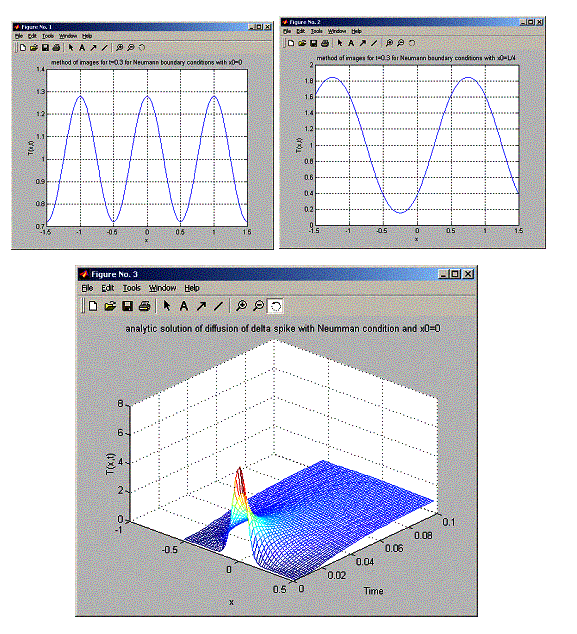
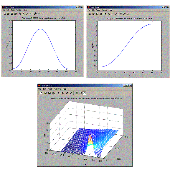
Problem 6.6 part C (part of HW 17)

Nasser Abbasi

Source code

function nma_problem_6_6_c()

%

% solves diffusion partial differential equation

% for Neumann bounday conditions. Problem 6.6 part C.

% Nasser Abbasi

help nma_problem_6_6_c; clear all; close all;

%

% First I plot the analytical solution for diffusion

% equation using method of images for Neumman bounday

% condition. The equation from Teacher's solution is

% T(x,t) = SUM Tg(x- (n L + (-1)^n x0),t)

% where Tg(x,t) = 1/sigma*sqrt(2 pi) exp(- (x-x0)^2 / (2 sigma^2 )

% i.e. the gaussian function.

% I plot the above for x0-0 and x0=L/4 at time some future time.

% This is so to compare the shape of the plot for that instance

% of time, with the FTCS method (which cover many instances of time).

tau = input('Enter time step in seconds:');

N = input('Enter number of space grid points:');

numberOfTimeSteps = input('Enter number of time steps:');

k = 1;

L = 1; % space distance total from -L/2 to L/2

x0 = 0; % where we want to find the solution at.

t=tau*numberOfTimeSteps/2; % picked time to calculate T using

% method of images to compare to

% analytic solution at the same time.

sigma = sqrt(2*k*t);

i = 0;

for(x= -1.5*L: 0.01*L : 1.5*L)

sum = 0;

for(n=-4:4)

gaussian = Tg( x- (n*L + (-1)^n *x0) ,x0,sigma);

sum = sum + gaussian ;

end

i=i+1;

T(i,1) = x;

T(i,2) = sum;

end

figure;

plot(T(:,1),T(:,2));

grid on;

title('method of images for t=0.3 for Neumann boundary conditions with x0=0');

xlabel('x');

ylabel('T(x,t)');

x0 = L/4; % where we want to find the solution at.

i=0;

for(x= -1.5*L: 0.01*L : 1.5*L)

sum = 0;

for(n=-4:4)

gaussian = Tg( x- (n*L + (-1)^n *x0) ,x0,sigma);

sum = sum + gaussian ;

end

i=i+1;

T(i,1) = x;

T(i,2) = sum;

end

figure;

plot(T(:,1),T(:,2));

grid on;

title('method of images for t=0.3 for Neumann boundary conditions with x0=L/4');

xlabel('x');

ylabel('T(x,t)');

%

% Now solve numerically for all time using FTCS

%

h = L/(N-2); % space distance between each point.

coeff = k * tau/h^2;

%

% set the variables to use for deciding to take

% snapshot for plotting.

%

numberOfPlots = 50; % number of snap shots

plotStep = numberOfTimeSteps/numberOfPlots;

plotNumber = 0;

%

% reserve space for the whole T(x,t) solution matrix

%

T= zeros(numberOfTimeSteps, N);

T(1,round(N/2)) = 1/h; % initial condition for delta at center

% part a

for( n = 1: numberOfTimeSteps - 1)

for( i = 2:N-1 )

T(n+1,i) = T(n,i) + coeff*( T(n,i+1) + T(n,i-1) - 2*T(n,i));

end

%

% set the Nuemann bounday conditions before

% next time step calculation of T

%

T(n+1,1) = T(n+1,2);

T(n+1,N) = T(n+1,N-1);

% periodicaly record T for plotting

if( rem(n,plotStep) < 1 )

plotNumber = plotNumber + 1;

finalT(plotNumber, :) = T(n,:);

timeVector(plotNumber) = n * tau;

end

end

%

% Now do the plots.

% set space vector as specificed by problem.

%

k=0;

for(i=0:N-1)

k = k+1;

spaceVector(k)= -L/2 + (i- (3/2) )*h;

end

figure;

mesh( spaceVector, timeVector, finalT );

title('analytic solution of diffusion of delta spike with Neumman condition and x0=0');

xlabel('x');

ylabel('Time');

zlabel('T(x,t)');

% now plot the T solution only at t to compare with the

% one from method of images above

figure;

plot(T(numberOfTimeSteps/2,:));

title(sprintf('T(x,t) at t=%1.5f, Neumman boundaries, for x0=0',t));

xlabel('x');

ylabel('T(x,t)');

%

% Now do the same thing, but at x0=L/4

%

%

% reserve space for the whole T(x,t) solution matrix

%

T= zeros(numberOfTimeSteps, N);

T(1,round(3*N/4)) = 1/h; % initial condition for delta at center

% part b, spike at x=0+L/4, since center

% at N/2. we put the spike at 3N/4

plotNumber = 0;

for( n = 1: numberOfTimeSteps - 1)

for( i = 2:N-1 )

T(n+1,i) = T(n,i) + coeff*( T(n,i+1) + T(n,i-1) - 2*T(n,i));

end

%

% set the Nuemman bounday conditions before

% next time step calculation of T

%

T(n+1,1) = T(n+1,2);

T(n+1,N) = T(n+1,N-1);

% periodicaly record T for plotting

if( rem(n,plotStep) < 1 )

plotNumber = plotNumber + 1;

finalT(plotNumber, :) = T(n,:);

timeVector(plotNumber) = n * tau;

end

end

figure;

mesh( spaceVector, timeVector, finalT );

title('analytic solution of diffusion of spike with Neumman condition and x0=L/4');

xlabel('x');

ylabel('Time');

zlabel('T(x,t)');

% now plot the T solution only at t to compare with the

% one from method of images above

figure;

plot(T(numberOfTimeSteps/2,:));

title(sprintf('T(x,t) at t=%1.5f, Neumman boundaries, for x0=L/4',t));

xlabel('x');

ylabel('T(x,t)');

%%%%%%%%%%%%%%%%%%%%%%%%%%%%%%%%%%%%%%%%%

% function to calculate the gaussian

%%%%%%%%%%%%%%%%%%%%%%%%%%%%%%%%%%%%%%%%%

function value=Tg(x,x0,sigma)

value = (x-x0);

value = value^2;

value = value / (2*sigma^2);

value = exp(- value);

term = sigma*sqrt(2*pi);

value = value * (1/term);

OUTPUT

» nma_problem_6_6_c

solves diffusion partial differential equation

for Neumann bounday conditions. Problem 6.6 part C.

Nasser Abbasi

Enter time step in seconds:1e-4

Enter number of space grid points:61

Enter number of time steps:1000

»