Problem 4.6 (a)

Nasser Abbasi

Source Code

function nma_HW_6_4

%

% nma_HW_6_4.m

% program to solve problem 6.4, page 201

% Nasser Abbasi

%

clear all; help nma_HW_6_4;

t= input('Enter the time to find the solution at in seconds:');

k= input('Enter value for k, thermal diffusion coefficient :');

L= input('Enter value for L:');

x0 = 0; % where we want to find the solution at.

sigma = sqrt(2*k*t);

i=0;

for(x= -1.5*L: 0.01*L : 1.5*L)

sum=0;

for(n=-4:4)

gaussian = Tg( (x+n*L) ,x0,sigma);

sum = sum + ( (-1)^n * gaussian ) ;

end

i=i+1;

T(i,1) = x;

% if( x <= (-L/2) | x > (L/2) )

% sum=0; % boundary condition

% end

T(i,2) = sum;

end

plot(T(:,1),T(:,2));

grid on;

%newXlabel=[-1.5:0.01:1.5];

%LINE=get(gca,'xtick');

%LINE=linspace(LINE(1),LINE(end),length(newXlabel));

%set(gca,'xtick',LINE);

%set(gca,'xticklabel',newXlabel);

newYlabel=[-2:1:2];

LINE=get(gca,'ytick');

LINE=linspace(LINE(1),LINE(end),length(newYlabel));

set(gca,'ytick',LINE);

set(gca,'yticklabel',newYlabel);

xlabel('X/L');

ylabel('T(x,t)');

%x0 = -1; % left image

%sigma = sqrt(2*k*t);

%i=0;

%for(x= -1.5*L: 0.01*L : 1.5*L)

% sum=0;

% for(n=-4:4)

% gaussian = Tg( (x+n*L) ,x0,sigma);

% sum = sum + ( (-1)^n * gaussian ) ;

% end

% i=i+1;

% T(i,1) = x;

% T(i,2) = sum;

%end

%hold on

%plot(T(:,1),T(:,2));

%%%%%%%%%%%%%%%%%%%%%%%%%%%%%%%%%%%%%%%%%

% function to calculate the gaussian

%%%%%%%%%%%%%%%%%%%%%%%%%%%%%%%%%%%%%%%%%

function value=Tg(x,x0,sigma)

value = (x-x0);

value = value^2;

value = value / (2*sigma^2);

value = exp(- value);

term = sigma*sqrt(2*pi);

value = value * (1/term);

OUTPUT

» nma_HW_6_4

nma_HW_6_4.m

program to solve problem 6.4, page 201

Nasser Abbasi

Enter the time to find the solution at in seconds:0.03

Enter value for k, thermal diffusion coefficient :1

Enter value for L:1

»

Dr:

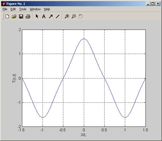
I can’t figure how to get the left and right images. I seem to have something wrong but can’t see it. When I use x0=0 and plot the T(x,t) I am getting the above, I was expecting to see the guassian shape extend to the sides over the x-axis, but not get the pull down below T=0 on the right and left. I went over the equation many times but do not see what I am doing wrong. I.e. the boundary conditions that T be zero outside –L/2 and L/2 are not being met automatically by the sum (equation 6.16). What Ami going wrong??

What is not clear to me, is if I needed to modify the equation for the boundary conditions or not.

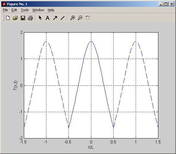
When I modified the program to plot each solution under different x0, i.e. the first for x0=0, then for x0=-1, then for x0=+1, This is what I get (and below it the modified program), again the ‘images’ are coming up upside down from the book. So I am really confused on this method, I think I do not understand this part well.

function nma_HW_6_4

%

% nma_HW_6_4.m

% program to solve problem 6.4, page 201

% Nasser Abbasi

%

clear all; help nma_HW_6_4;

t= input('Enter the time to find the solution at in seconds:');

k= input('Enter value for k, thermal diffusion coefficient :');

L= input('Enter value for L:');

x0 = 0; % where we want to find the solution at.

sigma = sqrt(2*k*t);

i=0;

for(x= -0.5*L: 0.01*L : 0.5*L)

sum=0;

for(n=-4:4)

gaussian = Tg( (x+n*L) ,x0,sigma);

sum = sum + ( (-1)^n * gaussian ) ;

end

i=i+1;

T(i,1) = x;

T(i,2) = sum;

end

plot(T(:,1),T(:,2));

grid on;

%newXlabel=[-1.5:0.01:1.5];

%LINE=get(gca,'xtick');

%LINE=linspace(LINE(1),LINE(end),length(newXlabel));

%set(gca,'xtick',LINE);

%set(gca,'xticklabel',newXlabel);

newYlabel=[-2:1:2];

LINE=get(gca,'ytick');

LINE=linspace(LINE(1),LINE(end),length(newYlabel));

set(gca,'ytick',LINE);

set(gca,'yticklabel',newYlabel);

xlabel('X/L');

ylabel('T(x,t)');

x0 = -1; % left image

sigma = sqrt(2*k*t);

i=0;

for(x= -1.5*L: 0.01*L : -0.5*L)

sum=0;

for(n=-4:4)

gaussian = Tg( (x+n*L) ,x0,sigma);

sum = sum + ( (-1)^n * gaussian ) ;

end

i=i+1;

T1(i,1) = x;

T1(i,2) = sum;

end

hold on

plot(T1(:,1),T1(:,2),'--');

x0 = 1; % right image

sigma = sqrt(2*k*t);

i=0;

for(x= 0.5*L: 0.01*L : 1.5*L)

sum=0;

for(n=-4:4)

gaussian = Tg( (x+n*L) ,x0,sigma);

sum = sum + ( (-1)^n * gaussian ) ;

end

i=i+1;

T2(i,1) = x;

T2(i,2) = sum;

end

hold on

plot(T2(:,1),T2(:,2),'--');

%%%%%%%%%%%%%%%%%%%%%%%%%%%%%%%%%%%%%%%%%

% function to calculate the gaussian

%%%%%%%%%%%%%%%%%%%%%%%%%%%%%%%%%%%%%%%%%

function value=Tg(x,x0,sigma)

value = (x-x0);

value = value^2;

value = value / (2*sigma^2);

value = exp(- value);

term = sigma*sqrt(2*pi);

value = value * (1/term);