Problem 5.27
Nasser Abbasi
Analysis and output
Modified the pendulum program to plot the power spectrum (and fourier transform) of the simple pendulum angular motion. This is an example of a run using small angle and one using a large angle:
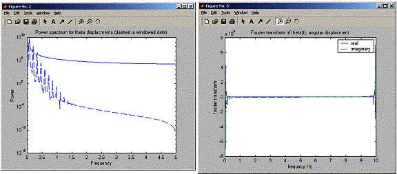
Large angle run:
»
nma_problem_5_27
problem_5_27 - Program to compute the motion
of a simple pendulum
and find the power spectrum for theta(t) (angular displacment)
time series.
modified from original pendul.m by Nasser
Abbasi to do
spectrum analysis.
Enter
initial angle (in degrees): 170
Enter
time step: 0.1
Enter
number of time steps: 1024
Turning
point at time t= 3.900000
Turning
point at time t= 11.500000
Turning
point at time t= 19.200000
Turning
point at time t= 26.900000
Turning
point at time t= 34.500000
Turning
point at time t= 42.200000
Turning
point at time t= 49.900000
Turning
point at time t= 57.500000
Turning
point at time t= 65.200000
Turning
point at time t= 72.900000
Turning
point at time t= 80.500000
Turning
point at time t= 88.200000
Turning
point at time t= 95.900000
Average period = 15.3333 +/- 0.0273115
»
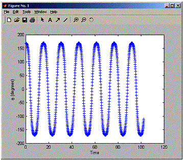
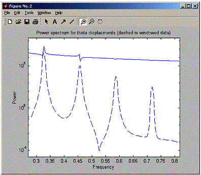
Now,
still in the large angle run, I used matlab zoom functionality to zoom more
into the part of the power spectrum and fourier transform to see the multiple
peaks, they can be clearly seen. Notice in the FFT, the peaks are there but not
as clear as in the power spectrum plot
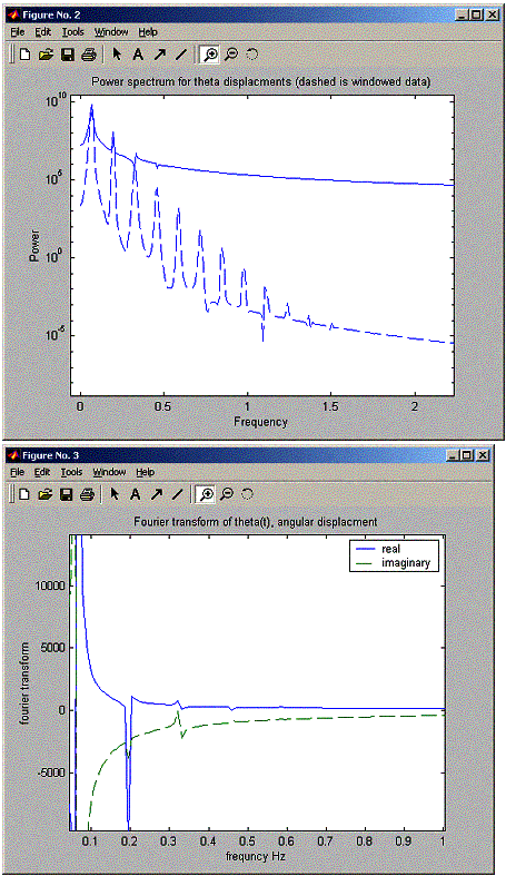
Now I run the program for a small angle to see the difference:
»
nma_problem_5_27
problem_5_27 - Program to compute the motion
of a simple pendulum
and find the power spectrum for theta(t) (angular displacment)
time series.
modified from original pendul.m by Nasser
Abbasi to do
spectrum analysis.
Enter
initial angle (in degrees): 20
Enter
time step: 0.1
Enter
number of time steps: 1024
Turning
point at time t= 1.600000
Turning
point at time t= 4.800000
Turning
point at time t= 8.000000
Turning
point at time t= 11.100000
Turning
point at time t= 14.300000
Turning
point at time t= 17.500000
Turning
point at time t= 20.600000
Turning
point at time t= 23.800000
Turning
point at time t= 26.900000
Turning
point at time t= 30.100000
Turning
point at time t= 33.300000
Turning
point at time t= 36.400000
Turning
point at time t= 39.600000
Turning
point at time t= 42.800000
Turning
point at time t= 45.900000
Turning
point at time t= 49.100000
Turning
point at time t= 52.300000
Turning
point at time t= 55.400000
Turning
point at time t= 58.600000
Turning
point at time t= 61.800000
Turning
point at time t= 64.900000
Turning
point at time t= 68.100000
Turning
point at time t= 71.200000
Turning
point at time t= 74.400000
Turning
point at time t= 77.600000
Turning
point at time t= 80.700000
Turning
point at time t= 83.900000
Turning
point at time t= 87.100000
Turning
point at time t= 90.200000
Turning
point at time t= 93.400000
Turning
point at time t= 96.600000
Turning
point at time t= 99.700000
Average
period = 6.32903 +/- 0.0171959
»
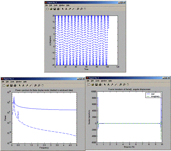
Again, use matlab zoom to look at closer:
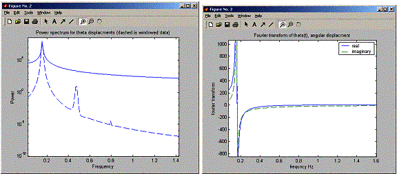
So, as the angle is increased we see side peaks show up. Now I need to answer the next question asking for the relation between the frequencies of these peaks.
The peaks look like they are spaced uniformally, at a distance of about 0.14 Hz from each others (when running for angle 170 degrees). The power of each peak becomes smaller at higher frequencies. At 2 Hz frequency, the peaks dissapeared. Noticed also that the windowed version of the data shows the peaks much more clearly.
I am not sure how to explain these peaks. Obvisouly the time series of the angular displacement of the pendulum shows it can be build from time serises of those made of those sub frequencies we see above. Equation 2.37 in the book shows the period of a simple pendulum as
![]()
so, since the period T is a function of the sin of the maximum angle, and using taylor expansion for the sin function, one can see that the period T can be expressed as a series expansion in terms of theta. Hence as we take more terms of the sum, we get closer to the actual period T. The peaks we see for the power spectrum of the angular displacement could be related to each partial sum of the series for the different periods depending on the length of the series taken?
Source code
%
problem_5_27 - Program to compute the motion of a simple pendulum
% and
find the power spectrum for theta(t)
(angular displacment)
% time
series.
%
modified from original pendul.m by Nasser Abbasi to do
%
spectrum analysis.
clear all; help nma_problem_5_27; % Clear the memory and print header
%* Set
initial position and velocity of pendulum
theta0 = input('Enter initial angle (in degrees): ');
theta =
theta0*pi/180; % Convert angle to radians
omega = 0; %
Set the initial velocity
%* Set
the physical constants and other variables
g_over_L = 1; %
The constant g/L
time = 0; % Initial time
irev = 0; %
Used to count number of reversals
tau = input('Enter time step: ');
%* Take
one backward step to start Verlet
accel =
-g_over_L*sin(theta); % Gravitational acceleration
theta_old = theta -
omega*tau + 0.5*tau^2*accel;
%* Loop
over desired number of steps with given time step
% and numerical method
nstep = input('Enter number of time steps: ');
for istep=1:nstep
%* Record angle and time for
plotting
t_plot(istep) = time;
th_plot(istep) = theta*180/pi;
% Convert angle to degrees
time = time + tau;
%* Compute new position and
velocity using
%
Euler or Verlet method
accel =
-g_over_L*sin(theta); % Gravitational acceleration
theta_new = 2*theta - theta_old + tau^2*accel;
theta_old = theta; % Verlet
method
theta = theta_new;
%* Test
if the pendulum has passed through theta = 0;
%
if yes, use time to estimate period
if(
theta*theta_old < 0 ) % Test position for sign change
fprintf('Turning point at time
t= %f \n',time);
if( irev == 0 ) % If
this is the first change,
time_old = time;
% just record the time
else
period(irev) = 2*(time - time_old);
time_old = time;
end
irev = irev + 1;
% Increment the number of reversals
end
end
%*
Estimate period of oscillation, including error bar
AvePeriod = mean(period);
ErrorBar =
std(period)/sqrt(irev);
fprintf('Average period = %g +/- %g\n',
AvePeriod,ErrorBar);
%* Graph
the oscillations as theta versus time
clf; figure(gcf); % Clear and forward figure
window
plot(t_plot,th_plot,'+');
xlabel('Time');
ylabel('\theta (degrees)');
%
% power
spectrum
%
f(1:nstep) =
(0:(nstep-1))/(tau*nstep); % Frequency scale
th_fft = fft(th_plot); % Fourier transform of z
displacement
th_spect =
abs(th_fft).^2; % Power spectrum of z displacement
%* Apply
the Hanning window to the time series and calculate
% the resulting power spectrum
window =
0.5*(1-cos(2*pi*((1:nstep)-1)/nstep)); %
Hanning window
th_w = th_plot' .*
window'; % Windowed time series
th_w_fft = fft(th_w); %
Fourier transf. (windowed data)
th_spectw =
abs(th_w_fft).^2; % Power spectrum (windowed data)
%* Graph
the power spectra for original and windowed data
figure;
semilogy(f(1:(nstep/2)),th_spect(1:(nstep/2)),'b-',...
f(1:(nstep/2)),th_spectw(1:(nstep/2)),'b--');
title('Power spectrum for theta displacments (dashed is
windowed data)');
xlabel('Frequency'); ylabel('Power');
%
% plot
the fourier transform of theta(t) to see the
%
frequncies
%
figure;
plot(f,real(th_fft),'-',f,imag(th_fft),'--');
legend('real','imaginary');
title('Fourier transform of theta(t), angular displacment');
ylabel('fourier transform');
xlabel('frequncy Hz');