Problem 5.23 (b)

By Nasser Abbasi

Output

» nma_sprfft

nma_sprfft - Program to compute the power spectrum of a

wilberforce pendulum. Modified from original sprfft

to solve problem 5.23(b), page 170.

Enter initial height (meter):0.1

input initial angle (degrees):0

Enter timestep: 0.1

»

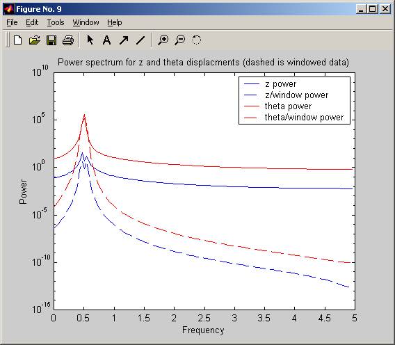
first I print the power spectrum for z and theta frequencies on the same plot. Notice that when frequency is 0.5 Hz, both z and theta frequencies contain the maximum power:

Next, plot the z transform and theta transforms to see the frequencies w_z and w_theta. (only the first half is shown):

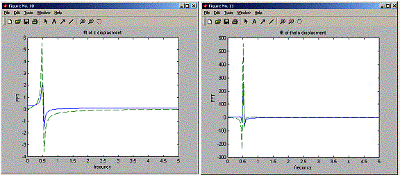
Notice that w_z and w_theta have frequency of 0.5 Hz.

When w_z = w_theta = w0, then normal mode frequencies w= w^2 +- sqrt(epsilon^2 / m*I)

Source code

% nma_sprfft - Program to compute the power spectrum of a

% wilberforce pendulum. Modified from original sprfft

% to solve problem 5.23(b), page 170.

%Nasser Abbasi

clear all; help nma_sprfft; % Clear memory and print header

%

% read parameters

%

z = input('Enter initial height (meter):');

v = 0;

theta = input('input initial angle (degrees):');

theta = theta*pi/180; %convert to radian

omega = 0;

tau = input('Enter timestep: ');

mass = 0.5; % kg

Inert = 1.0e-4; % rotatioal inertia (kg m^2)

k_spr = 5.0; % spring constant

delta = 1.0e-3; %torsional spring constant N m

epsil = 1.0e-2; %coupling constant N

param = [mass Inert k_spr delta epsil];

%

% MAIN LOOP

%

time=0;

zplot(1) = z*100; % z in cm

thplot(1) = theta;

tplot(1) = time;

iplot = 2;

nstep= 256;

for(i=1:nstep)

%

% save the time series for z,v,theta,omega

% for later analysis, fft, etc...

%

z_timeSeries(i) = z;

v_timeSeries(i) = v;

theta_timeSeries(i) = theta;

omega_timeSeries(i) = omega;

state = [z v theta omega];

state = rk4(state,time,tau,'f3_13',param);

time = time+tau;

z = state(1);

v = state(2);

theta = state(3);

omega = state(4);

end

% Calculate the power spectrum of the time series for vertical

% displacment

f(1:nstep) = (0:(nstep-1))/(tau*nstep); % Frequency

z_fft = fft(z_timeSeries); % Fourier transform of z displacement

z_spect = abs(z_fft).^2; % Power spectrum of z displacement

%* Apply the Hanning window to the time series and calculate

% the resulting power spectrum

window = 0.5*(1-cos(2*pi*((1:nstep)-1)/nstep)); % Hanning window

z_w = z_timeSeries' .* window'; % Windowed time series

zw_fft = fft(z_w); % Fourier transf. (windowed data)

z_spectw = abs(zw_fft).^2; % Power spectrum (windowed data)

%* Graph the power spectra for original and windowed data

figure;

semilogy(f(1:(nstep/2)),z_spect(1:(nstep/2)),'b-',...

f(1:(nstep/2)),z_spectw(1:(nstep/2)),'b--');

title('Power spectrum for z and theta displacments (dashed is windowed data)');

xlabel('Frequency'); ylabel('Power');

%

% now plot the same for the angular frequncy.

%

theta_fft = fft(theta_timeSeries); % Fourier transform of angle

theta_spect = abs(theta_fft).^2; % Power spectrum of angle

%* Apply the Hanning window to the time series and calculate

% the resulting power spectrum

theta_w = theta_timeSeries' .* window'; % Windowed time series

thetaw_fft = fft(theta_w); % Fourier transf. (windowed data)

theta_spectw = abs(thetaw_fft).^2; % Power spectrum (windowed data)

hold on;

semilogy(f(1:(nstep/2)),theta_spect(1:(nstep/2)),'r-',...

f(1:(nstep/2)),theta_spectw(1:(nstep/2)),'r--');

legend('z power','z/window power','theta power','theta/window power');

%

% plot the fft for both z and theta time series

%

figure;

plot(f(1:(nstep/2)),real(z_fft(1:(nstep/2))),'-',...

f(1:(nstep/2)),imag(z_fft(1:(nstep/2))),'--');

title('fft of z displacment');

xlabel('frequncy');

ylabel('FFT');

figure;

plot(f(1:(nstep/2)),real(theta_fft(1:(nstep/2))),'-',...

f(1:(nstep/2)),imag(theta_fft(1:(nstep/2))),'--');

title('fft of theta displacment');

xlabel('frequncy');

ylabel('FFT');

function deriv = f3_13(a,time,param)

%

% teacher f3_13 function used to solve problem

% 5.20(b)

%

z=a(1);

v=a(2);

theta=a(3);

omega=a(4);

mass=param(1);

Inert=param(2);

k_spr=param(3);

delta = param(4);

epsil= param(5);

deriv(1)= v;

deriv(2)= (-k_spr*z -0.5*epsil*theta)/mass;

deriv(3)=omega;

deriv(4)=(-delta*theta - 0.5*epsil*z)/Inert;

return;