Problem 5.20
By Nasser Abbasi
OUTPUT
»
nma_problem_5_20
program to solve problem 5.20
analysis of filtering effects.
Nasser Abbasi
Enter
the number of sin signals to combine:5
enter
frequncy for the 1 sin signal (HZ):0.1
enter
frequncy for the 2 sin signal (HZ):0.2
enter
frequncy for the 3 sin signal (HZ):0.3
enter
frequncy for the 4 sin signal (HZ):1.2
enter
frequncy for the 5 sin signal (HZ):1.3
Will
use 6.5 Hz as the sampling frequncy, sample interval=0.153846 seconds
enter
number of points to sample:100
Max
power in the combined signal before filtering is 2516.21, min power is 0.528981
Max
power in the combined signal after low pass filter is 2434.95, min power is
3.04936e-031
Max
power in the combined signal after high pass filter is 869.33, min power is
3.15544e-030
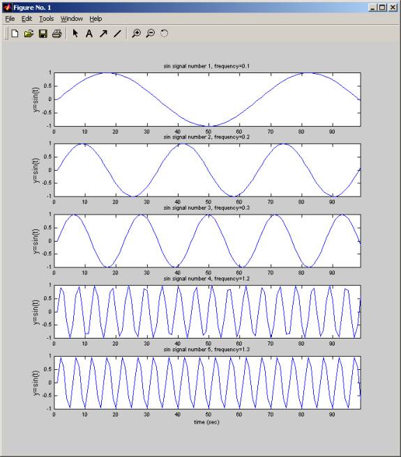
In
this plot the each of the signals are plotted as a time series, before
combining:
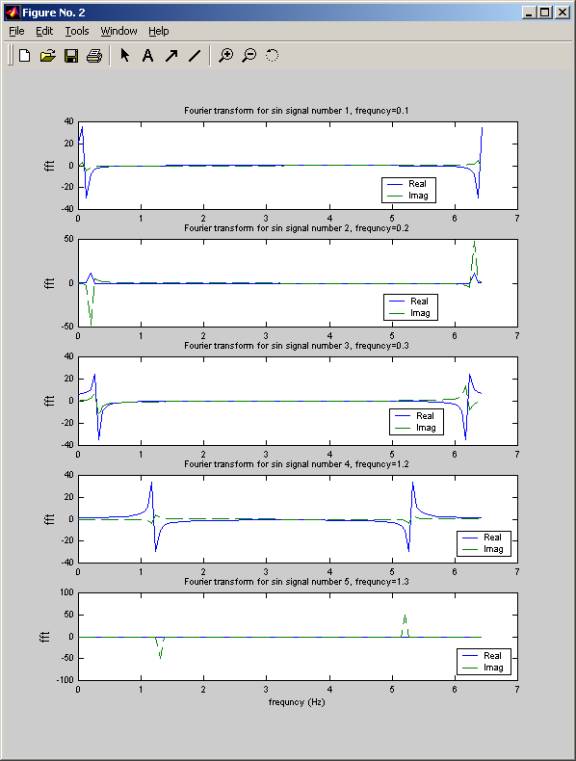
This this plot, I show the fourier transform of each
signal
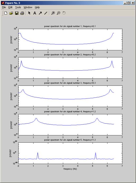
In this plot I show the power spectrum (unnormalized)
of each signal
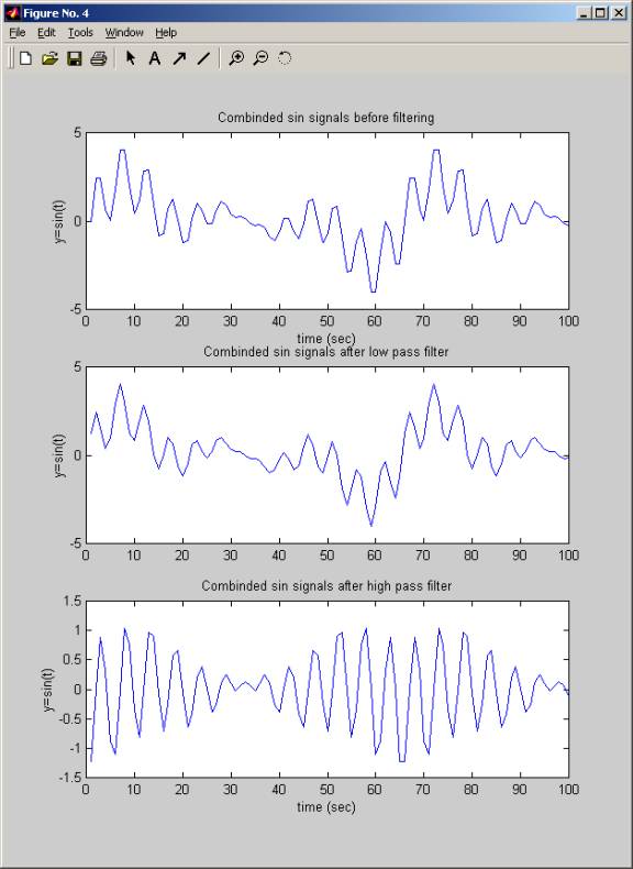
In this plot I show the time series of the signals,
after being combinded but before filtering, then after applying the low-pass
and the high-filters.
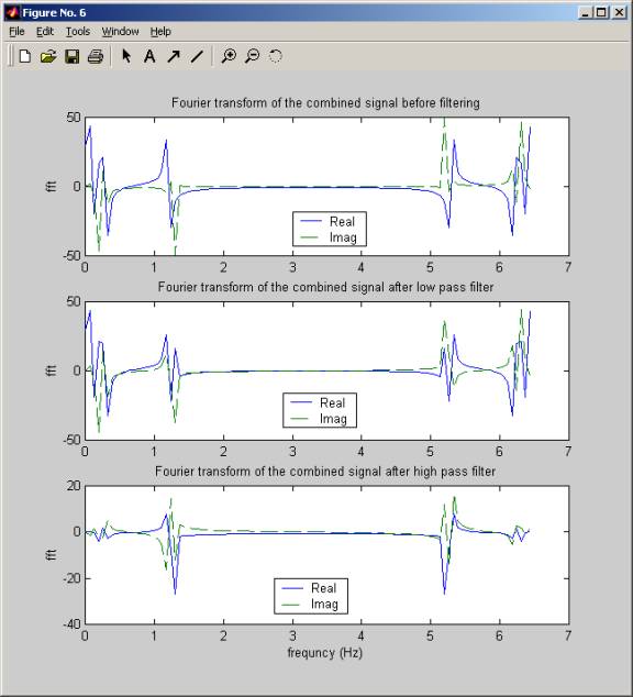
This plots shows the fourier transforms for the combined signal before filtering, and then the fourier transform after the low-pass and high-pass filters applied to the combined signal. Notice for the low-pass filter, the fourier transform for the 2 higher frequencies are smaller than in the original combined signal. Notice in the fourier transform for the high-pass filter, the low frequencies having smaller magnitude than in the original combined signal.
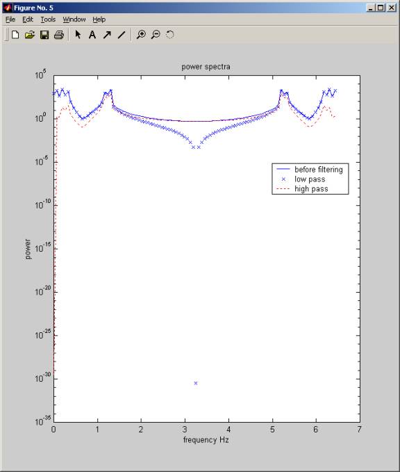
In this plot, I show the power spectrum of the
combined signal, and on the same plot the power spectrum for both the low-pass
and high-pass signals. To see clearly what happened, I use matlab zoom to zoom
in closer (see next plot)
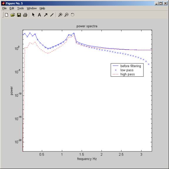
This
is the same plot as the above, but zoomed in more closely. Here we see clearly
that the low-pass signal (the cross x) has the same power as the original
combined signal when the frequencies are low. But the high-pass signal (the red
dashed lines) has much lower power for the same low frequencies.
Notice that for large frequencies the reverse happened. The low pass signal have less power at those high frequencies, while the high-pass signal now matches the original combined signal, and have high power at thos frequencies.
This
means that the low-pass filter allowed low frequencies to pass in while
blocking high frequencies, and the high-pass filter allowed high frequencies to
pass in while blocking low frequencies.
source code
%
%
program to solve problem 5.20
%
analysis of filtering effects.
% Nasser
Abbasi
%
%
%
overall logic: Ask the user to enter how many
%
signals they want to analyse. Get the freuqncy for
% each,
the number of points to sample from each.
%
% find
the maximum frequncy to be used, and use an
%
interval such that the sampling frequncy is 5 times
% as
large as the largest frequncy from the above user input.
% (used
5 times to get more continuos effect. I only need
% to be
2 times more than the highest frequency).
%
% Next,
find the time signal for each, then add the signals
%
togother, next smooth the combined signal using the filters
% given
in the problem. Next find the power spectrum for
% the
result, and show that the filter acts as either a low
% pass
or high pass filter by showing that either only low
%
frequncies or high frequncies are kept in the filtered signal.
%
%
clear all; help
nma_problem_5_20;
numberOfSignals = input('Enter the number of sin signals to combine:');
if(numberOfSignals
<= 0 )
return;
end
for(i=1:numberOfSignals)
S=sprintf('enter frequncy for the
%d sin signal (HZ):',i);
freq(i)= input(S);
end
sampleFrequncy =
5*max(freq);
tau = 1/sampleFrequncy;
fprintf('Will use %g Hz as the sampling frequncy, sample
interval=%g seconds\n',...
sampleFrequncy,tau);
N = input('enter number of points to sample:');
t = 0:(N-1);
t = t * tau; %[0
tau 2tau 3tau ....]
f = (0:(N-1))/(N*tau); % the frequncies x-axis for fft and power spectra
%
% note:
feval returns a row vector.
% each
row of signal matrix contains one time series.
% for
different sin signal
%
figure;
for(i=1:numberOfSignals)
temp = feval('sin',2*pi*freq(i)*t);
signal(i,:) = temp(1,:);
subplot(numberOfSignals,1,i);
plot(signal(i,:));
title(sprintf('sin signal number
%d, frequency=%g',i,freq(i)),...
'fontsize',7);
ylabel('y=sin(t)');
axis([0 N-1 -1 1]);
set(gca,'fontsize',7);
end
% put an
x label to the bottom plot only to save space between plots
% since
all the plots x-axis is the same.
xlabel('time (sec)');
%
% plot
the fft of all signals
% that
we combined above into one, this is just to help
% me
understand what is going on at the end.
%
figure;
for(i=1:numberOfSignals)
subplot(numberOfSignals,1,i);
fft_ = fft(signal(i,:));
plot(f,real(fft_),'-',f,imag(fft_),'--');
title(sprintf('Fourier transform
for sin signal number %d, frequncy=%g',i,freq(i)),...
'fontsize',7);
ylabel('fft');
set(gca,'fontsize',7);
legend('Real','Imag',4);
end
xlabel('frequncy (Hz)');
%
% plot
the power spectra of all signals
% that
we combined above into one, this is just to help
% me
understand what is going on at the end.
%
figure;
for(i=1:numberOfSignals)
subplot(numberOfSignals,1,i);
fft_ =
fft(signal(i,:));
powerSpectra = abs(fft_).^2;
semilogy(f,powerSpectra,'-');
title(sprintf('power spectrum for
sin signal number %d, frequncy=%g',i,freq(i)),...
'fontsize',7);
ylabel('power');
set(gca,'fontsize',7);
end
xlabel('frequncy (Hz)');
%
% sum
all the signals from above into one
% row
vector
%
for(i=1:N)
sumSignal(1,i) = sum(signal(:,i)); %
not sure of I should average or not
%
the total sum by divide on numberOfSignals;
end
%
% start
a new figure that contains the combined signal
% before
and after smoothing
%
figure;
subplot(3,1,1);
plot(sumSignal);
title('Combinded sin signals before filtering');
xlabel('time (sec)');
ylabel('y=sin(t)');
%
% now
filter the combined time signal
%
% padd a
point at the end of combined signal to make it easy
% to
average the points. Use y(N+1)= y(1) to padd
%
tempSignal = [sumSignal
sumSignal(1)];
%
% Now
lets apply the filters
%
for(j=1:N)
low_z(j) =
(tempSignal(j) + tempSignal(j+1)) /2;
high_z(j) = (tempSignal(j) - tempSignal(j+1)) /2;
end
%
% plot
the filtered combined signal
%
subplot(3,1,2);
plot(low_z);
title('Combinded sin signals after low pass filter');
ylabel('y=sin(t)');
subplot(3,1,3);
plot(high_z);
title('Combinded sin signals after high pass filter');
xlabel('time (sec)');
ylabel('y=sin(t)');
%
% find
power spectra for the sumSignal (i.e. y)
% to
find the power spectra, we first find the fourier
%
transform for y
yt=fft(sumSignal);
powerSpectra = abs(yt).^2;
figure;
semilogy(f,powerSpectra,'-');
title('power spectra');
ylabel('power');
fprintf('Max power in the combined signal before filtering is
%g, min power is %g\n',...
max(powerSpectra),min(powerSpectra));
%
% find
and plot the power spectra for the filtered signal
%
low_zt = fft(low_z);
powerSpectra =
abs(low_zt).^2;
hold on;
semilogy(f,powerSpectra,'x');
fprintf('Max power in the combined signal after low pass filter
is %g, min power is %g\n',...
max(powerSpectra),min(powerSpectra));
high_zt=fft(high_z);
powerSpectra =
abs(high_zt).^2;
semilogy(f,powerSpectra,'r:');
xlabel('frequency Hz');
fprintf('Max power in the combined signal after high pass
filter is %g, min power is %g\n',...
max(powerSpectra),min(powerSpectra));
legend('before filtering','low
pass','high pass');
%
% plot
the fourier transforms for combined signal
% and
for the filtered signal
%
figure;
subplot(3,1,1);
plot(f,real(yt),'-',f,imag(yt),'--');
title('Fourier transform of the combined signal before
filtering');
ylabel('fft');
legend('Real','Imag',4);
subplot(3,1,2);
plot(f,real(low_zt),'-',f,imag(low_zt),'--');
title('Fourier transform of the combined signal after low
pass filter');
ylabel('fft');
legend('Real','Imag',4);
subplot(3,1,3);
plot(f,real(high_zt),'-',f,imag(high_zt),'--');
title('Fourier transform of the combined signal after high
pass filter');
ylabel('fft');
xlabel('frequncy (Hz)');
legend('Real','Imag',4);