HW 4.18
Nasser Abbasi, California State Univ, San Jose.
Physics 240, Spring 2002.
Question
Consider a particle in a quantum square well potential of
depth ![]() and half width
and half width ![]() . The energy eignvalues,
. The energy eignvalues, ![]() , are given by the transcendental equation
, are given by the transcendental equation
![]()
for the even states and
![]()
for the odd states. Write a program to obtain the first 10
energy eigenvalues of an electron for ![]() and
and ![]() where
where ![]() is the Bohr radius.
is the Bohr radius.
Solution
Notes:
|
Table 1. SI
base units |
|||||||||||||||||||||||||||||
|
|
|
|||||||||||||||||||||||||||
|
|
|
|
|||||||||||||||||||||||||||
|
Derived quantity |
Name |
Symbol |
|
area |
square meter |
m2 |
|
volume |
cubic meter |
m3 |
|
speed, velocity |
meter per second |
m/s |
|
acceleration |
meter per second squared |
m/s2 |
|
wave number |
reciprocal meter |
m-1 |
|
mass density |
kilogram per cubic meter |
kg/m3 |
|
specific volume |
cubic meter per kilogram |
m3/kg |
|
current density |
ampere per square meter |
A/m2 |
|
magnetic field strength |
ampere per meter |
A/m |
|
amount-of-substance concentration |
mole per cubic meter |
mol/m3 |
|
luminance |
candela per square meter |
cd/m2 |
|
mass fraction |
kilogram per kilogram, which may be represented by the
number 1 |
kg/kg = 1 |
|
|
||
![]() ,
and h=6.626 10-34 joule sec or h = 4.136 x 10⁻¹⁵ eV s
,
and h=6.626 10-34 joule sec or h = 4.136 x 10⁻¹⁵ eV s
![]() also called cot(a).
also called cot(a).
ao =
5.29177×10⁻¹¹ m
Mass of an electron is 9.11*10-31 kg, note that 1 eV = 1.782 661 731 x 10-36 kg
So, the mass of an electron is
9*10^-31 / 1.782661731x10^-36 = 5.048630283296300* 10^5 eV
Electron
carries a precise charge of 1.6*10-19 coulombs
the electron volt
(ev). It is the energy gained by an electron (or proton, same size of electric
charge) moving through a voltage difference of one volt.
The SI unit for energy is the JOULE. 1 eV = 1.602
x 10-19 joule.
So, V is our example is –13.6 x 1.602 x 10^-19 J.
Bohr
radius = 5.291772083 × 10⁻¹¹ m
OUTPUT
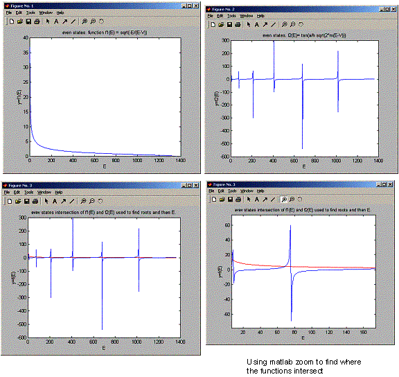
For even states, I first plot the functions ![]() and function
and function ![]()
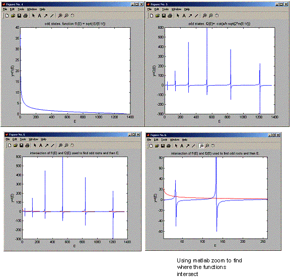
The intersection of the above two functions, gives the values that can be used to find E.
I first did this problem with plots. I used matlab to plot
the above 2 functions on the same plot. Then zoomed in to find the exact value
on the y-axis. Then used the function f1 above to find E (since I know V). i.e.
when I find the y-axis value, i.e. f1, then I used it to solve ![]() for E. i.e.
for E. i.e. ![]()
These are the values for E for even states using this hand graphical/zoom method:
-13.541, -13.516, -12.916, -11.7, -9.415
All in eV.
For the odd states, these are the states I found using this method:
-13.2948, -13.2668, -12.3831, -10.88
But I need to solve this using a program!, so next I looked at it this way:
Solve for f1-f2=0.
i.e.

Is the equation I need to solve for even states.
For odd states, 
I use newton’s method for solve for the above 2 equations.
The program asks the user if they want to solve for odd or even states, then at first it plots f1 and f2, and then plots f1 and f2 on the same plot. Then it asks the user for a guess to start looking for a root.
For even states:

For odd states

» nma_HW_4_18
even or odd states root finding? [1=odd, 2=even]:2
found a root at E=-13.5239
E now is -13.5139
found a root at E=-12.9154
E now is -12.9054
found a root at E=-12.9154
E now is -12.9054
found a root at E=-12.9154
E now is -12.9054
found a root at E=-12.9154
E now is -12.9054
found a root at E=-12.9154
E now is -12.9054
found a root at E=-12.9154
E now is -12.9054
found a root at E=-12.9154
E now is -12.9054
found a root at E=-12.9154
E now is -12.9054
found a root at E=-12.9154
»
» nma_HW_4_18
even or odd states root finding? [1=odd, 2=even]:1
found a root at E=-10.8691
E now is -10.8591
found a root at E=-10.8691
E now is -10.8591
found a root at E=-10.8691
E now is -10.8591
found a root at E=-10.8691
E now is -10.8591
found a root at E=-10.8691
E now is -10.8591
found a root at E=-10.8691
E now is -10.8591
found a root at E=-10.8691
E now is -10.8591
found a root at E=-10.8691
E now is -10.8591
found a root at E=-10.8691
E now is -10.8591
found a root at E=-10.8691
»
Source code
function nma_HW_4_18()
%
program to solve problem 4.18, to find the first 10 energy
%
eigenvalues of an electron in quantum square well.
%
% Nasser
Abbasi, San Jose State Univ. Phys 240
%
numberOfRootsFound=0;
a0=5.29177*(10^-11);
a=20*a0;
% plank
bar constant in J.sec
h=6.626*(10^-34)/(2*pi);
% in eV
%h=
4.136*(10^-15)/(2*pi)
%mass of
electron in kg
m=9.11*(10^-31);
%ground
enegry level, in Joules
V=-13.6*1.602*(10^-19);
plotFunctions;
state = input('even or odd states root finding? [1=odd, 2=even]:');
guessIncrement = 0.01 *
1.602e-19;
if(
state == 2 )
E = V + guessIncrement;
i=0;
numberOfRootsFound=0;
while( 1 )
i=i+1;
E_last=E;
E = E_last - ( f(E_last)
/ df(E_last) );
if( E==E_last )
fprintf('found a root at
E=%g\n',E/(1.602e-19));
numberOfRootsFound = numberOfRootsFound + 1;
if( numberOfRootsFound ==
10 )
break;
else
%
% use the last root found as estimate
to find next root
% after adding small increment to it.
%
E = E + guessIncrement;
fprintf('E now is %g\n',E/(1.602e-19));
end
end
i=i+1;
if( i > 50000)
break;
end
end
else
E = V + guessIncrement;
i=0;
numberOfRootsFound=0;
while( 1 )
i=i+1;
E_last=E;
E = E_last - (
f_odd(E_last) / df_odd(E_last) );
if( E==E_last )
fprintf('found a root at
E=%g\n',E/(1.602e-19));
numberOfRootsFound =
numberOfRootsFound + 1;
if( numberOfRootsFound ==
10 )
break;
else
%
% use the last root found as estimate
to find next root
% after adding small
increment to it.
%
E = E + guessIncrement;
fprintf('E now is %g\n',E/(1.602e-19));
end
end
i=i+1;
if( i > 50000)
break;
end
end
end
%%%%%%%%%%%%%%%%%%%%%%%%%%%
%
function y=f()
%
%%%%%%%%%%%%%%%%%%%%%%%%%%%
function y=f(E)
a0=5.29177*(10^-11);
a=20*a0;
h=6.626*(10^-34)/(2*pi);
m=9.11*(10^-31);
V=-13.6*1.602*(10^-19);
y=-sqrt(-E/(E-V)) + tan(a/h*2^(1/2)*(m*(E-V))^(1/2)) ;
%%%%%%%%%%%%%%%%%%%%%%%%%%%%
%
function yp=df()
%
%%%%%%%%%%%%%%%%%%%%%%%%%%%%%
function yp=df(E)
a0=5.29177*(10^-11);
a=20*a0;
h=6.626*(10^-34)/(2*pi);
m=9.11*(10^-31);
V=-13.6*1.602*(10^-19);
yp=-1/2/(-E/(E-V))^(1/2)*(-1/(E-V)+E/(E-V)^2)+...
1/2*(1+tan(a/h*2^(1/2)*(m*(E-V))^(1/2))^2)*a/h*2^(1/2)/(m*(E-V))^(1/2)*m;
%%%%%%%%%%%%%%%%%%%%%%%%%%%
%
function y=fodd()
%
%%%%%%%%%%%%%%%%%%%%%%%%%%%
function y=f_odd(E)
a0=5.29177*(10^-11);
a=20*a0;
h=6.626*(10^-34)/(2*pi);
m=9.11*(10^-31);
V=-13.6*1.602*(10^-19);
y=-sqrt(-E/(E-V)) - cot(a/h*2^(1/2)*(m*(E-V))^(1/2)) ;
%%%%%%%%%%%%%%%%%%%%%%%%%%%%
%
function yp=df_odd()
%
%%%%%%%%%%%%%%%%%%%%%%%%%%%%%
function yp=df_odd(E)
a0=5.29177*(10^-11);
a=20*a0;
h=6.626*(10^-34)/(2*pi);
m=9.11*(10^-31);
V=-13.6*1.602*(10^-19);
yp= -1/2/(-E/(E-V))^(1/2)*(-1/(E-V)+E/(E-V)^2)-...
1/2*(-1-cot(a/h*2^(1/2)*(m*(E-V))^(1/2))^2)*a/h*2^(1/2)/(m*(E-V))^(1/2)*m;
%%%%%%%%%%%%%%%%%%%
%
%%%%%%%%%%%%%%%%%%%%
function plotFunctions()
a0=5.29177*(10^-11);
a=20*a0;
% plank
bar constant in J.sec
h=6.626*(10^-34)/(2*pi);
% in eV
%h=
4.136*(10^-15)/(2*pi)
%mass of
electron in kg
m=9.11*(10^-31);
V= -13.6*1.602e-19;
E= V;
i=0;
while(1);
E=E+ (0.01*1.602e-19);
if( E>=0)
break;
end;
i=i+1;
f1(i)= sqrt( -E/(E-V) );
end
figure;
plot(f1);
title('even states. function f1(E)
= sqrt(-E/(E-V))');
xlabel('E');
ylabel('y=f1(E)');
E=V;
i=0;
f2=[];
while(1)
E=E+ (0.01 * 1.602e-19);
i=i+1;
f2(i)=tan( (a/h) * sqrt(2*m*(E-V)));
if( E>=0 )
break;
end
end
figure;
plot(f2,'-');
title('even states. f2(E)= tan(a/h
sqrt(2*m(E-V)))');
xlabel('E');
ylabel('y=f2(E)');
figure;
plot(f1,'r');
hold on;
plot(f2,'b');
title('evev states intersection of
f1(E) and f2(E) used to find roots and then E.');
xlabel('E');
ylabel('y=f(E)');
%
% now plot
the odd states functions
%
E= V;
i=0;
while(1);
E=E+ (0.01*1.602e-19);
if( E>=0)
break;
end;
i=i+1;
f1(i)= sqrt( -E/(E-V) );
end
figure;
plot(f1);
title('odd states. function f1(E) =
sqrt(-E/(E-V))');
xlabel('E');
ylabel('y=f1(E)');
E=V;
i=0;
f2=[];
while(1)
E=E+ (0.01 * 1.602e-19);
i=i+1;
f2(i)=-cot( (a/h) * sqrt(2*m*(E-V)));
if( E>=0 )
break;
end
end
figure;
plot(f2,'-');
title('odd states. f2(E)= -cot(a/h
sqrt(2*m(E-V)))');
xlabel('E');
ylabel('y=f2(E)');
figure;
plot(f1,'r');
hold on;
plot(f2,'b');
title('intersection of f1(E) and
f2(E) used to find odd roots and then E.');
xlabel('E');
ylabel('y=f(E)');