The indexing method used is that described in the class.
Symbolic generating of system equations for 2D regular grid for solving Laplace equation using finite difference method
By Nasser M. Abbasi
updated oct 28,2010
Introduction
When solving ![]() ) using finite difference method, in order to make it easy to see the internal structure of the A matrix using the standard 5 points Laplacian scheme, the following is a small function which generates the symbolic format of these equations for a given N, the number of grid points on one edge. At the end of this note, the system equations are generated for N=4,5,6,7,8. One can see the form of the A matrix with the dominant diagonal and the corresponding bands. It is mostly a sparse matrix.
) using finite difference method, in order to make it easy to see the internal structure of the A matrix using the standard 5 points Laplacian scheme, the following is a small function which generates the symbolic format of these equations for a given N, the number of grid points on one edge. At the end of this note, the system equations are generated for N=4,5,6,7,8. One can see the form of the A matrix with the dominant diagonal and the corresponding bands. It is mostly a sparse matrix.
The indexing method used is that described in the class.
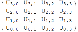
Define U at each grid point
In[59]:=

Out[61]=
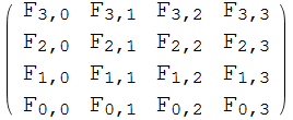
Define the force vector
In[62]:=
![]()
Out[63]=
In[64]:=

In[67]:=

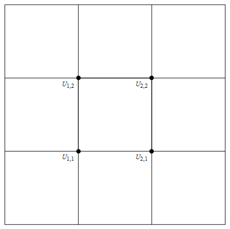
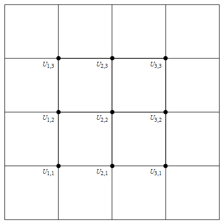
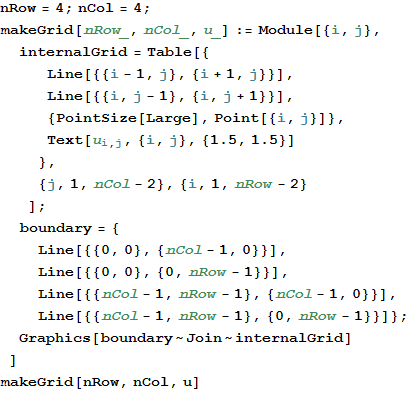
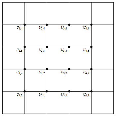
Draw the grid with the unknown above at each point
In[68]:=
Out[70]=
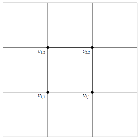
Generate the discrete equations at each of the internal grid points
In[71]:=
![]()
Out[72]=
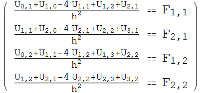
List the unknowns
In[73]:=
![]()
Out[73]=

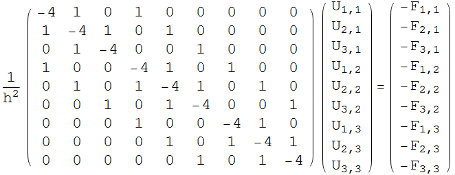
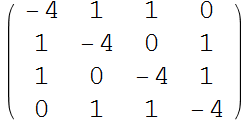
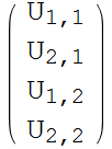
Generate the equations of the form AU=F
In[80]:=

Out[82]=
 |
 |
= | 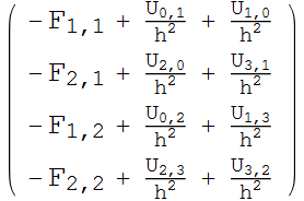 |
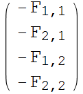
For homegenous Boundary conditions
In[83]:=

Out[85]=
 |
 |
= |  |
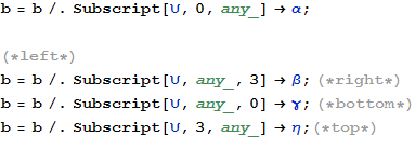
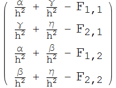
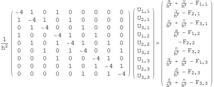
set the boundary conditions. Assume left side is U=α,Right side U=β, bottom side U=γ, top side U=η, then the above becomes
In[86]:=
Display the equations again
In[90]:=
![]()
Out[90]=
 |
 |
= |  |
Now the system can be solved for the unknowns U , given the force F values.
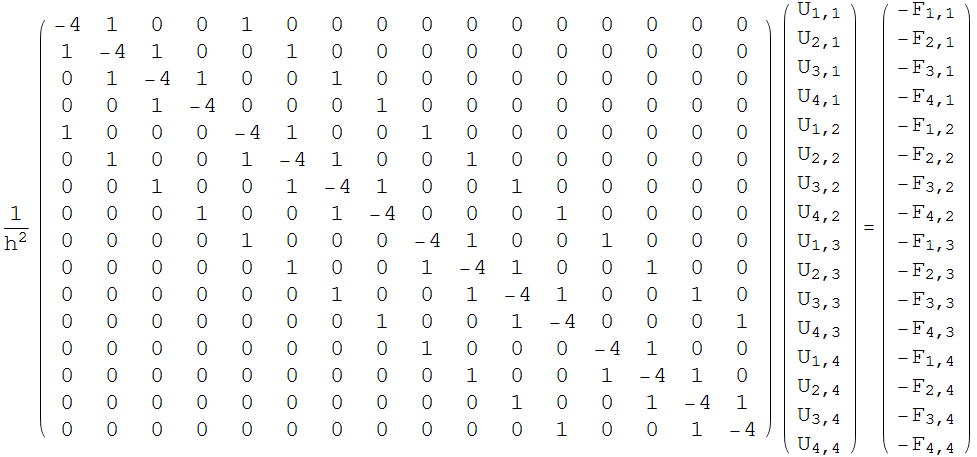
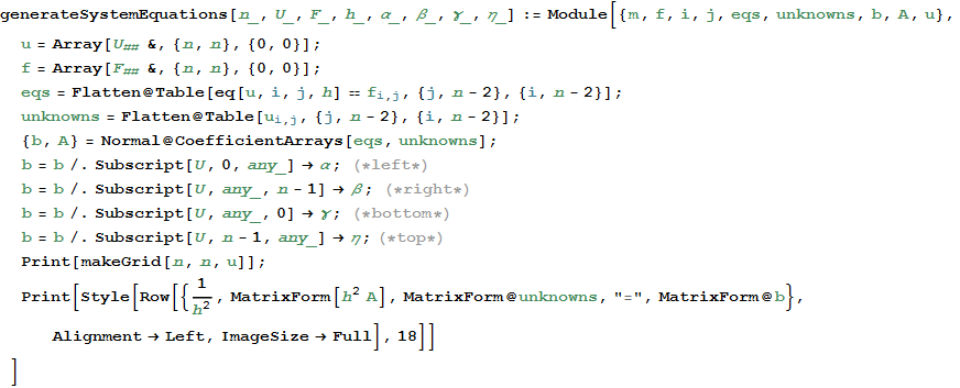
Below is the system equations generated for N=3,4,5,6,7,8. Put the above code into one function to use it all the time
In[91]:=
In[92]:=



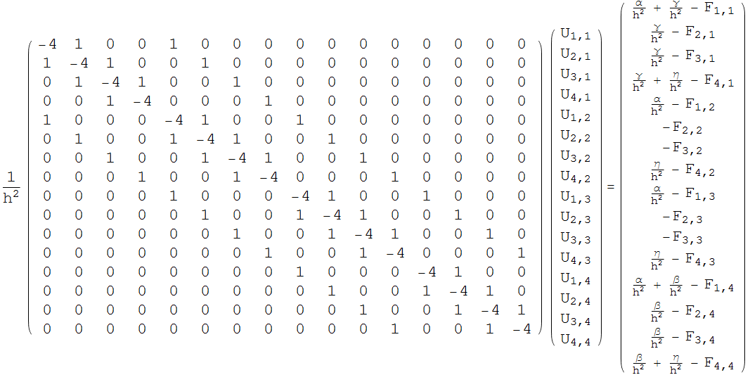

For homogenous boundary conditions
In[94]:=

