The goal of this project is to analyze and compare different numerical methods for solving the first order advection PDE.
Following the analytical analysis for stability of the numerical scheme, animation were done to visually illustrate and confirm these results. This was carried for different parameters. The animation was programmed in Mathematica and saved to animated gif files which was then loaded into the HTML version of this report.
Fortran 95 was used for the computation part, while Mathematica was used for the animation and graphics part.
The above link contains all the supporting material for the project, including the Fortran program (in source and windows executable format) used to carry the main computation, and the Mathematica program used to do the animation and the Unix bash file used to process the computation for different parameters.
The specific PDE example used for the analysis and animation was the one provided by Professor Donald Dabdub for the final exam for his MAE 185 course (Numerical methods for mechanical engineers) in spring 2006. This PDE is described below:
Solve numerically\[ \frac {\partial c}{\partial t} + u \frac {\partial c}{\partial x} = 0 \]
Where \(c(x,t)\) is the concentration of a given material as a function of time and space.
The above is solved for the following 2 cases
The problem parameters are:
\begin {align*} t & \geq 0\\ 0 & \leq x\leq L \end {align*}
Where \(L=100\ \text {feet.}\). Initial conditions are \[ c\left ( x,0\right ) =F\left ( x\right ) =\left \{ \begin {array} [c]{ccc}1+\cos \left ( \pi \left ( \frac {x-30}{5}\right ) \right ) & & 25\leq x\leq 25\\ 0 & & \text {otherwise}\end {array} \right . \]
The boundary conditions are
\begin {align*} c\left ( 0,t\right ) & =0\\ c(L,t) & =0 \end {align*}
This PDE is an example of an IBVP (Initial and Boundary Value Problem).
Different numerical methods are used to solve the above PDE. The methods are compared for stability using Von Neumann stability analysis.
The numerical methods are also compared for accuracy. This was done by comparing the numerical solution to the known analytical solution at each time step. The comparison was done by computing the root mean square error (RMSE) between the numerical and the analytical solution at each time step.
The method with the least RMSE at the end of the simulation is considered the most accurate.
The above PDE has a known analytical solution which is \[ C\left ( x,t\right ) =F\left ( x-ut\right ) \]
The above analytical solution indicates that the initial concentration will move from left to right with the advection speed \(u\).
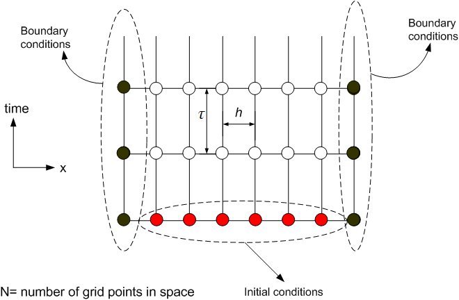
The formulation of each numerical method is shown below. \(h\) is used to represent \(\Delta x,\) the space between 2 space grid point, or the space step size, and \(\tau \) is used to represent \(\Delta t,\) the time step.
The space line has \(N\) grid points. The spacing \(h\) was fixed at \(0.01\) ft for all the methods and for all the test cases, while \(\tau \) was changed. This made comparing the different methods simpler. The following diagram illustrates the discretization used.
Should we consider the lower left and the lower right grid points above as part of the initial conditions, or part of the boundary conditions?
Stability of each method is derived. Stability is important, since by the Lax-Richtmyer equivalence theorem1, stability implies convergence of the solution. Convergence of the numerical solutions implies that as the step size becomes smaller, the numerical solution converges to the analytical solution.
Explicit and implicit numerical methods are used. When solving for the future value of the solution at a single node in terms of only past values, the method is called an explicit method. In other words, when the only unknown is the future value of the solution at a single node, and everything else on the right hand side of the finite difference equation is a solution derived at earlier time step, the method is explicit.
An implicit method is one in which the finite difference equation contains the solution at a at future time at more than one node. In other words, future solution are being solved for at more than one node in terms of the solution at earlier time. Implicit methods therefor are usually solved by matrix methods by solving \(Ax=b\) where \(b\) represents present present known solution values, and \(x\) are the unknown future solution values, and \(A\) is the coefficient matrix which will usually be block diagonal (or tri diagonal) in shape.
In the derivations below, the notation of \(C_{i}^{n}\) is used to indicate the solution at time step \(n\) and at space node \(i.\) Hence \(C\left ( x_{i},t_{n}\right ) \) is written as \(C_{i}^{n}\). This notation seems to be more clear than the \(C_{i,n}\) notation.
Different finite difference schemes for solving a PDE are obtained by using different methods of approximating the derivative terms in the PDE.
This will be illustrated using the space derivative \(\frac {\partial c}{\partial x}.\) This derivative can be approximated in one of the following 3 ways (all at time step \(n\))
\[ \frac {\partial c}{\partial x}\approx \frac {C_{i}^{n}-C_{i-1}^{n}}{h}\ \ \]
\[ \frac {\partial c}{\partial x}\approx \frac {C_{i+1}^{n}-C_{i}^{n}}{h}\ \ \]
\[ \frac {\partial c}{\partial x}\approx \frac {C_{i+1}^{n}-C_{i-1}^{n}}{2h}\]
The following are the derivation of a number of methods for solving the advection PDE obtained by using the above definitions for the derivative when applied to both space and time.
With FTCS, the forward time derivative, and the centered space derivative are used. Hence the advection PDE can be written as
\begin {equation} \frac {C_{i}^{n+1}-C_{i}^{n}}{\tau }=-u\left ( \frac {C_{i+1}^{n}-C_{i-1}^{n}}{2h}\right ) \tag {0} \end {equation}
Solving for \(C_{i}^{n+1}\) results in
\begin {equation} \fbox {$C_{i}^{n+1}=C_{i}^{n}-\frac {u\tau }{2h}\left ( C_{i+1}^{n}-C_{i-1}^{n}\right ) $} \tag {1} \end {equation}
This method will be shown to be unconditionally unstable.
Here, the forward time derivative for\(\frac {\partial C}{\partial t}\) is used and also the forward space derivative for\(\frac {\partial C}{\partial x}\). This results in
\[ \frac {C_{i}^{n+1}-C_{i}^{n}}{\tau }=-u\left ( \frac {C_{i+1}^{n}-C_{i}^{n}}{h}\right ) \]
\[ \fbox {$C_{i}^{n+1}=C_{i}^{n}-\frac {u\tau }{h}\left ( C_{i+1}^{n}-C_{i}^{n}\right ) $}\]
This method will be shown to be unconditionally unstable as well.
Here, the forward time derivative for \(\frac {\partial C}{\partial t}\) is used, and the backward derivative for \(\frac {\partial C}{\partial x}\) is used. This results in
\[ \frac {C_{i}^{n+1}-C_{i}^{n}}{\tau }=-u\left ( \frac {C_{i}^{n}-C_{i-1}^{n}}{h}\right ) \]
\[ \fbox {$C_{i}^{n+1}=C_{i}^{n}-\frac {u\tau }{h}\left ( C_{i}^{n}-C_{i-1}^{n}\right ) $}\]
This will be shown to be stable if \(\frac {u\tau }{h}\leq 1\)
Looking at the FTCS eq (1) above, and shown below again
\[ C_{i}^{n+1}=C_{i}^{n}-\frac {u\tau }{2h}\left ( C_{i+1}^{n}-C_{i-1}^{n}\right ) \]
The term \(C_{i}^{n}\) above is replaced by its average value\(\frac {C_{i+1}^{n}+C_{i-1}^{n}}{2}\) to obtain the LAX method
\begin {equation} \fbox {$C_{i}^{n+1}=\frac {1}{2}\left ( C_{i+1}^{n}+C_{i-1}^{n}\right ) -\frac {u\tau }{2h}\left ( C_{i+1}^{n}-C_{i-1}^{n}\right ) $} \tag {4} \end {equation}
This method will be shown to be stable if \(\frac {u\tau }{h}\leq 1\)
By using the second-order finite difference scheme for the time derivative, the method of Lax-Wendroff method is obtained
\[ C_{i}^{n+1}=C_{i}^{n}-\frac {u\tau }{2h}\left ( C_{i+1}^{n}-C_{i-1}^{n}\right ) +\frac {u^{2}\tau ^{2}}{2h^{2}}\left ( C_{i+1}^{n}+C_{i-1}^{n}-2C_{i}^{n}\right ) \]
In this method, the centered derivative is used for both time and space. This results in
\[ \fbox {$\frac {C_{i}^{n+1}-C_{i}^{n-1}}{2\tau }=-u\left ( \frac {C_{i+1}^{n}-C_{i-1}^{n}}{2h}\right ) $}\]
This method requires a special starting procedure due to the term \(C_{i}^{n-1}\). Another scheme such as Lax can be used to kick start this method.
Given the explicit FTCS derived above
\[ \frac {C_{i}^{n+1}-C_{i}^{n}}{\tau }=-u\left ( \frac {C_{i+1}^{n}-C_{i-1}^{n}}{2h}\right ) \]
The above is modified it by evaluating the space center derivative at time step \(n+1\) instead of at time step \(n\), this results in
\begin {equation} \frac {C_{i}^{n+1}-C_{i}^{n}}{\tau }=-u\left ( \frac {C_{i+1}^{n+1}-C_{i-1}^{n+1}}{2h}\right ) \tag {5A} \end {equation}
Hence
\begin {equation} \fbox {$C_{i}^{n+1}+\frac {u\tau }{2h}C_{i+1}^{n+1}-\frac {u\tau }{2h}C_{i-1}^{n+1}=C_{i}^{n}$} \tag {5B} \end {equation}
Writing it in matrix form, first letting \(\alpha =\frac {u\tau }{2h}\) results in
\[\begin {bmatrix} 1 & 0 & 0 & 0 & \cdots & 0 & 0\\ -\alpha & 1 & \alpha & 0 & \cdots & 0 & 0\\ 0 & -\alpha & 1 & \alpha & \cdots & 0 & 0\\ 0 & 0 & -\alpha & 1 & \alpha & \cdots & 0\\ \vdots & & & & & & \\ 0 & 0 & 0 & 0 & 0 & 0 & 1 \end {bmatrix}\begin {bmatrix} C_{0}^{n+1}\\ C_{1}^{n+1}\\ C_{2}^{n+1}\\ C_{3}^{n+1}\\ \vdots \\ C_{N-1}^{n+1}\end {bmatrix} =\begin {bmatrix} C_{0}^{n}\\ C_{1}^{n}\\ C_{2}^{n}\\ C_{3}^{n}\\ \vdots \\ C_{N-1}^{n}\end {bmatrix} \]
Where \(N\) is the number of space grid points.
The above is written as \[ Ax=b \]
Solving for \(x,\) which represents the solution at time step \(n+1\) or at time \(t=\left ( n+1\right ) \tau \). \(b\) represents the current solution at time step \(n\), and \(A\) is the matrix of the coefficients shown above.
Due to the form of the \(A\) matrix, (Called tri diagonal, or Block diagonal), an algorithm that takes advantages of this form is used. This is called the Thomas algorithm. This greatly speeds up the solution. If we had used a general algorithm to solve this system such as the Gauss elimination method, it would have been much slower, making the implicit method not practical to use. (Some tests on the same data showed the Thomas algorithm to be 50 times faster than Gaussian elimination).
This method uses center difference for the derivative around the space step \(\left ( i+\frac {1}{2}\right ) h\) and the time step \(\left ( n+\frac {1}{2}\right ) \tau \)
This leads to the following scheme
\[ \fbox {$\left ( 1-\frac {u\tau }{h}\right ) C_{i}^{n+1}+\left ( 1+\frac {u\tau }{h}\right ) C_{i+1}^{n+1}=\left ( 1+\frac {u\tau }{h}\right ) C_{i}^{n}+\left ( 1-\frac {u\tau }{h}\right ) C_{i+1}^{n}$}\]
This can also be solved using similar matrix method to that used for the implicit FTCS. This method is not used in this report.
By taking the average of the explicit FTCS and the implicit FTCS formulations (shown again below), the C-N scheme is derived
\[ \frac {C_{i}^{n+1}-C_{i}^{n}}{\tau }=-u\left ( \frac {C_{i+1}^{n}-C_{i-1}^{n}}{2h}\right ) \]
\[ \frac {C_{i}^{n+1}-C_{i}^{n}}{\tau }=-u\left ( \frac {C_{i+1}^{n+1}-C_{i-1}^{n+1}}{2h}\right ) \]
Taking the average of the above results in
\[ \frac {C_{i}^{n+1}-C_{i}^{n}}{\tau }=-\frac {u}{2}\left ( \frac {C_{i+1}^{n}-C_{i-1}^{n}}{2h}\right ) -\frac {u}{2}\left ( \frac {C_{i+1}^{n+1}-C_{i-1}^{n+1}}{2h}\right ) \]
\[ \fbox {$C_{i}^{n+1}+\frac {u\tau }{4h}C_{i+1}^{n+1}-\frac {u\tau }{4h}C_{i-1}^{n+1}=C_{i}^{n}-\frac {u\tau }{4h}C_{i+1}^{n}+\frac {u\tau }{4h}C_{i-1}^{n}$}\]
Now the system \(Ax=b\) is setup to solve for future values as follows. Let \(\alpha =\frac {u\tau }{4h}\), the system can be written as
\[\begin {bmatrix} 1 & 0 & 0 & 0 & 0 & 0\\ -\alpha & 1 & \alpha & 0 & 0 & 0\\ 0 & -\alpha & 1 & \alpha & 0 & 0\\ 0 & 0 & -\alpha & 1 & \alpha & 0\\ 0 & 0 & 0 & -\alpha & 1 & 0\\ 0 & 0 & 0 & 0 & 0 & 1 \end {bmatrix}\begin {bmatrix} C_{0}^{n+1}\\ C_{1}^{n+1}\\ C_{2}^{n+1}\\ C_{3}^{n+1}\\ \vdots \\ C_{N-1}^{n+1}\end {bmatrix} =\begin {bmatrix} C_{0}^{n}\\ C_{1}^{n}-\alpha C_{2}^{n}+\alpha C_{0}^{n}\\ C_{2}^{n}-\alpha C_{3}^{n}+\alpha C_{1}^{n}\\ C_{3}^{n}-\alpha C_{4}^{n}+\alpha C_{2}^{n}\\ \vdots \\ C_{N-1}^{n}\end {bmatrix} \]
Thomas algorithm is used to solve the above system for \(C_{i}^{n+1}.\)
A numerical solution is stable if the "energy content" remain below some limiting value no matter how long the solution is integrated. In essence, this means that the solution does not ’blow up’ after some time. This can be called BIBO stability (Bounded In Bounded Out).
Hence one way to analyze the stability of the numerical solution is to determine an expression that relates the amplitude of the solution between 2 time steps, and to determine if this ratio remain less than or equal to a unity as more and more time steps are taken.
This type of analysis is called Von Neumann stability analysis for numerical methods.
The analysis is based of finding an expression for the magnification factor of the wave amplitude at each step. The solution will be stable if this magnification factor is less than one.
Let the magnification factor be \(\xi \). The numerical scheme is stable iff\[ \left \vert \zeta \right \vert \leq 1 \]
The Courant–Friedrichs–Lewy (CFL) criteria for stability says that \[ \left \vert \zeta \right \vert \leq 1\Leftrightarrow \left \vert \frac {u\tau }{h}\right \vert \leq 1 \]
Where \(u,h,\) and \(\tau \) are as defined above: \(u\) is the wave speed, \(h=\Delta x\) and \(\tau =\Delta t.\)
The number \(\frac {u\tau }{h}\) is also called the courant number.
Some numerical methods will be shown to be unconditionally unstable (such as explicit FTCS and the explicit upwind). This means that even if courant number was \(\leq 1\), the numerical solutions will eventually become unstable.
Some explicit methods such as LAX, are conditionally stable if the courant number was \(\leq 1.\)
Implicit methods are unconditionally stable, hence courant number is not used for these methods. However, this does not mean one can take as large step as one wants with the implicit methods, since accuracy will be affected even if the solution remain stable.
Hence, the best numerical scheme is one in which the largest step size can be taken, with the least amount of inaccuracy in the numerical solution while remaining stable.
For numerical scheme that are conditionally stable, it can be seen from the CFL condition that for a fixed speed \(u\) and fixed \(h\), the maximum time step that can be taken is given by
\[ \tau _{\max }\leq \frac {h}{u}\]
It can be immediately seen from above, that for the case when the advection speed is varying and is a function of time such as the case when \(u\left ( t\right ) =\frac {t}{20}\) implying that the speed is increasing with time, then when using a fixed time step \(\tau \) it will eventually become larger than \(\frac {h}{u}\) and the numerical scheme will be unstable. This is because as \(u\left ( t\right ) \) is becoming larger and larger, while \(h\) is fixed, the term \(\frac {h}{u}\) will become smaller and smaller.
Hence to keep the courant number \(\frac {u\tau }{h}\leq 1\) , the time step taken must remain less than \(\frac {h}{u}\), hence using a fixed time step with increasing \(u\) will eventually lead to instability.
This will affect the explicit methods that are conditionally stable such as the LAX method, since the Lax method is explicit and depends on satisfying the CFL all the time for its stability. Implicit methods are stable for any time step.
In the following we derive the details of the stability analysis and use Von Neumann analysis to derive an expression for the amplification factor \(\zeta \) for different numerical schemes.
So to summarize:
Using Von Neumann method, the following trial solution to the PDE is assumed\[ c\left ( x,t\right ) =A\left ( t\right ) e^{jkx}\] where \(j=\sqrt {-1}\) and \(k\) is the wave number and \(A\) is the amplitude of the wave, as a function of time.
Hence the solution at time step \(n\) and at \(x=x_{i}=ih\) is written as
\begin {equation} A^{n}e^{jkih} \tag {2} \end {equation}
Substitute this trial solution (2) into the (1) results in
\begin {equation} A^{n+1}e^{jkih}=A^{n}e^{jkih}-\frac {u\tau }{2h}\left ( A^{n}e^{jk\left ( i+1\right ) h}-A^{n}e^{jk\left ( i-1\right ) h}\right ) \tag {3} \end {equation}
Let \(\xi \) be the ratio of the amplitude of the wave at time step \(n+1\) relative to that at time step \(n\). hence \[ \xi =\frac {A^{n+1}}{A^{n}}\]
Divide (3) by \(A^{n}\) results in
\[ \xi e^{jkih}=e^{jkih}-\frac {u\tau }{2h}\left ( e^{jk\left ( i+1\right ) h}-e^{jk\left ( i-1\right ) h}\right ) \]
Divide the above by \(e^{jkih}\)
\begin {align*} \xi & =1-\frac {u\tau }{2h}\left ( e^{jkh}-e^{-jkh}\right ) \\ & =1-\frac {u\tau }{h}j\sin \left ( kh\right ) \end {align*}
Hence \[ \left \vert \xi \right \vert =\sqrt {1+\left ( \frac {u\tau }{h}\sin \left ( kh\right ) \right ) ^{2}}\]
This implies that \(\left \vert \xi \right \vert \geq 1\) regardless of the time step \(\tau \) selected or the space step \(h\), hence \[ \fbox {FTCS is unconditionally unstable.}\]
For a fixed speed \(u\), the instability can be delayed by making \(\frac {\tau }{h}\) smaller, but it could not be prevented. Eventually this numerical solution will blow up. This will be illustrated below in an animation. See case 3 and 4 as examples.
The instability can be delayed by making \(\tau \) smaller for a fixed \(h,\) or by making \(h\) larger for a fixed \(\tau \).
\[ C_{i}^{n+1}=C_{i}^{n}-\frac {u\tau }{h}\left ( C_{i+1}^{n}-C_{i}^{n}\right ) \]
Substitute the trial solution \(A^{n}e^{jkih}\) into the above
\begin {align*} A^{n+1}e^{jkih} & =A^{n}e^{jkih}-\frac {u\tau }{h}\left ( A^{n}e^{jk\left ( i+1\right ) h}-A^{n}e^{jkih}\right ) \\ \xi & =1-\frac {u\tau }{h}\left ( e^{jkh}-1\right ) \\ & =1+\frac {u\tau }{h}-\frac {u\tau }{h}e^{jkh}\\ & =1+\frac {u\tau }{h}-\frac {u\tau }{h}\left ( \cos \left ( kh\right ) +j\sin \left ( kh\right ) \right ) \\ & =1+\frac {u\tau }{h}\left ( 1-\cos kh\right ) -j\frac {u\tau }{h}\sin kh \end {align*}
Let \(\frac {u\tau }{h}=\lambda \)
Hence
\[ \xi =1+\lambda \left ( 1-\cos kh\right ) -j\lambda \sin kh \]
\begin {align*} \left \vert \xi \right \vert ^{2} & =\left ( 1+\lambda \left ( 1-\cos kh\right ) \right ) ^{2}+\left ( \lambda \sin kh\right ) ^{2}\\ & =1+2\lambda \left ( 1-\cos kh\right ) +\lambda ^{2}\left ( 1-\cos kh\right ) ^{2}+\lambda ^{2}\sin ^{2}kh\\ & =1+2\lambda \left ( 1-\cos kh\right ) +\lambda ^{2}\left ( 1-2\cos kh+\cos ^{2}kh\right ) +\lambda ^{2}\sin ^{2}kh\\ & =1+2\lambda -2\lambda \cos kh+\lambda ^{2}-2\lambda ^{2}\cos kh+\lambda ^{2}\cos ^{2}kh+\lambda ^{2}\sin ^{2}kh\\ & =1+2\lambda -2\lambda \cos kh+2\lambda ^{2}-2\lambda ^{2}\cos kh\\ & =1+2\lambda \left ( 1+\lambda \right ) \left ( 1-\cos kh\right ) \end {align*}
Hence for stability it is required that \[ \left \vert 1+2\lambda \left ( 1+\lambda \right ) \left ( 1-\cos kh\right ) \right \vert \leq 1 \]
or
\[ 2\lambda \left ( 1+\lambda \right ) \left ( 1-\cos kh\right ) \leq 0 \]
since \(\lambda =\frac {u\tau }{h}\), a positive quantity, then the above condition can not be satisfied. Hence the downwind method is unconditionally unstable.
\[ C_{i}^{n+1}=C_{i}^{n}-\frac {u\tau }{h}\left ( C_{i}^{n}-C_{i-1}^{n}\right ) \]
Substitute the trial solution \(A^{n}e^{jkih}\) into the above
\begin {align*} A^{n+1}e^{jkih} & =A^{n}e^{jkih}-\frac {u\tau }{h}\left ( A^{n}e^{jkih}-A^{n}e^{jk\left ( i-1\right ) h}\right ) \\ \xi & =1-\frac {u\tau }{h}\left ( 1-e^{-jkh}\right ) \\ & =1-\frac {u\tau }{h}+\frac {u\tau }{h}e^{-jkh}\\ & =1-\frac {u\tau }{h}+\frac {u\tau }{h}\left ( \cos \left ( kh\right ) -j\sin \left ( kh\right ) \right ) \\ & =1-\frac {u\tau }{h}\left ( 1-\cos kh\right ) -j\frac {u\tau }{h}\sin kh \end {align*}
Let \(\frac {u\tau }{h}=\lambda \)
Hence
\[ \xi =1-\lambda \left ( 1-\cos kh\right ) -j\lambda \sin kh \]
Hence
\begin {align*} \left \vert \xi \right \vert ^{2} & =\left ( 1-\lambda \left ( 1-\cos kh\right ) \right ) ^{2}+\left ( \lambda \sin kh\right ) ^{2}\\ & =1-2\lambda \left ( 1-\cos kh\right ) +\lambda ^{2}\left ( 1-\cos kh\right ) ^{2}+\lambda ^{2}\sin ^{2}kh\\ & =1-2\lambda +2\lambda \cos kh+\lambda ^{2}\left ( 1+\cos ^{2}kh-2\cos kh\right ) +\lambda ^{2}\sin ^{2}kh\\ & =1-2\lambda +2\lambda \cos kh+\lambda ^{2}+\lambda ^{2}\cos ^{2}kh-2\lambda ^{2}\cos kh+\lambda ^{2}\sin ^{2}kh\\ & =1-2\lambda +2\lambda \cos kh+2\lambda ^{2}-2\lambda ^{2}\cos kh\\ & =1-2\lambda \left ( 1-\lambda \right ) \left ( 1-\cos kh\right ) \end {align*}
Hence for stability it is required that
\[ \left \vert 1-2\lambda \left ( 1-\lambda \right ) \left ( 1-\cos kh\right ) \right \vert \leq 1 \]
or
\[ -2\lambda \left ( 1-\lambda \right ) \left ( 1-\cos kh\right ) \leq 0 \]
Which will be true only if \(\left ( 1-\lambda \right ) \geq 0\) or \(\lambda \leq 1\) hence this implies
\[ \frac {u\tau }{h}\leq 1 \]
Hence the upwind method is stable if the CFL condition is satisfied. This will be seen as the same stability condition for the Lax method below.
Replace the trial function from (2) in Lax formulation in (4) and obtain
\[ A^{n+1}e^{jkih}=\frac {1}{2}\left ( A^{n}e^{jk\left ( i+1\right ) h}+A^{n}e^{jk\left ( i-1\right ) h}\right ) -\frac {u\tau }{2h}\left ( A^{n}e^{jk\left ( i+1\right ) h}-A^{n}e^{jk\left ( i-1\right ) h}\right ) \]
Divide by \(A^{n}e^{jkih}\) , the magnification factor \(\zeta \) is obtained
\begin {align*} \zeta & =\frac {1}{2}\left ( e^{jkh}+e^{-jkh}\right ) -\frac {u\tau }{2h}\left ( e^{jkh}-e^{-jkh}\right ) \\ & =\cos \left ( kh\right ) -j\frac {u\tau }{h}\sin \left ( kh\right ) \end {align*}
Hence
\[ \left \vert \zeta \right \vert =\sqrt {\cos ^{2}\left ( kh\right ) +\left ( \frac {u\tau }{h}\right ) ^{2}\sin ^{2}\left ( kh\right ) }\]
Since \(\cos ^{2}\left ( kh\right ) \leq 1\) and \(\sin ^{2}\left ( kh\right ) \leq \) \(1\), then it is seen that \(\left \vert \zeta \right \vert \leq 1\) if \(\frac {u\tau }{h}\leq 1\)
Hence the following is the condition for stability \[ \tau \leq \frac {h}{u}\]
As mentioned earlier, this is called the CFL condition.
The Lax method is stable for \(\tau \leq \frac {h}{u}\) however, a modified version of this method is more accurate, which is the Lax-Wendroff method.
This is the same as the Lax method. The method is stable if \(\tau \leq \frac {h}{u}\)
Replace the trial function from (2) in (5B) results in
\[ A^{n+1}e^{jkih}+\frac {u\tau }{2h}A^{n+1}e^{jk\left ( i+1\right ) h}-\frac {u\tau }{2h}A^{n+1}e^{jk\left ( i-1\right ) h}=A^{n}e^{jkih}\]
Divide by \(A^{n}e^{jkih}\)
\begin {align*} \xi +\frac {u\tau }{2h}\xi e^{jkh}-\frac {u\tau }{2h}\xi e^{-jkh} & =1\\ \xi \left ( 1+\frac {u\tau }{2h}e^{jkh}-\frac {u\tau }{2h}e^{-jkh}\right ) & =1\\ \xi \left ( 1+j\frac {u\tau }{h}\sin \left ( kh\right ) \right ) & =1\\ \xi & =\frac {1}{1+j\frac {u\tau }{h}\sin \left ( kh\right ) }=\frac {1-j\frac {u\tau }{h}\sin \left ( kh\right ) }{1+\frac {u\tau }{h}\sin \left ( kh\right ) } \end {align*}
Hence \[ \left \vert \xi \right \vert =\frac {\sqrt {1+\left ( \frac {u\tau }{h}\right ) ^{2}\sin ^{2}\left ( kh\right ) }}{1+\frac {u\tau }{h}\sin \left ( kh\right ) }<1 \]
Hence this shows that the \[ \fbox {Implicit FTCS\ method is unconditionally stable.}\]
This property is common to all implicit methods.
Even though the implicit FTCS is stable, it is not very accurate. See case 8 below for an example.
For the Fortran implementation, the following methods are implemented. The explicit FTCS, Explicit Lax, Implicit FTCS, and Implicit Crank-Nicolson.
For each method, the following was generated
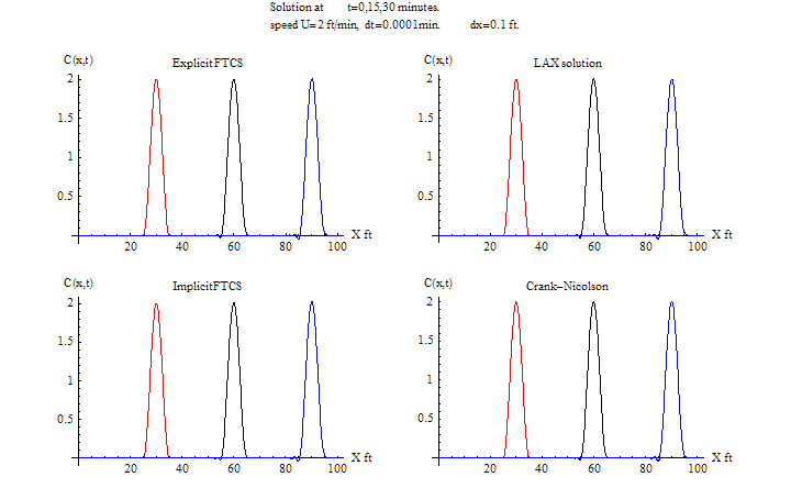
To compare the stability and accuracy of the methods, the time step was changed (increased) and a new run was made. 8 different values of time steps are used. So there are 8 tests cases. These 8 test cases were run for both fixed speed \(\left ( u=2\text { ft/min}\right ) \) and for \(u=\frac {t}{20}\) ft/min.
This table below summarizes these cases. The appendix contains all the plots. The animations are added as HTML links.
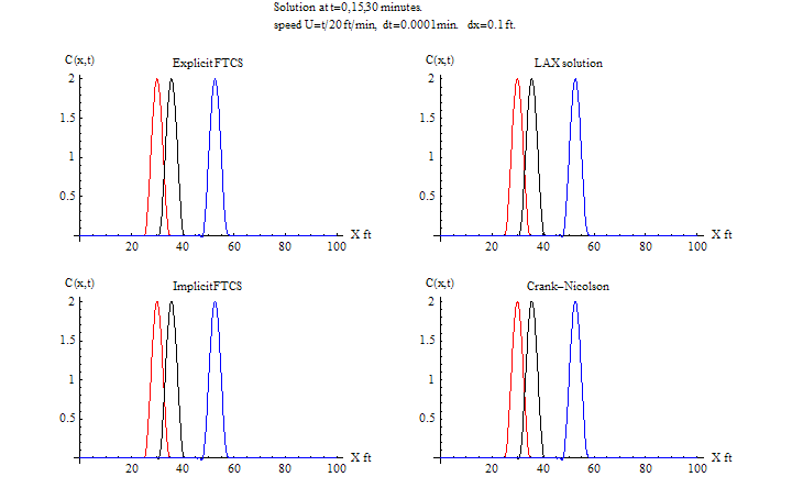
\(\tau =0.0001\) sec, \(h=0.1\ ft\)
Note the following: The explicit FTCS remained stable throughout the run due to the small time step. All other methods were stable as well during the run. For the CPU for the varying \(u\) case, notice that for the implicit methods this value is larger than the CPU for the same methods but when \(u\) is fixed. This is due to the fact that the matrix \(A\) is no longer constant, and must be recomputed at each time step before calling Thomas algorithm to solve \(Ax=b\) system.
Also notice that the CPU time for the implicit methods is larger than the explicit methods. This is due to the extra computational cost in solving \(Ax=b\). Even when using Thomas algorithm, this is still more expensive than the explicit methods when number of time steps is large.
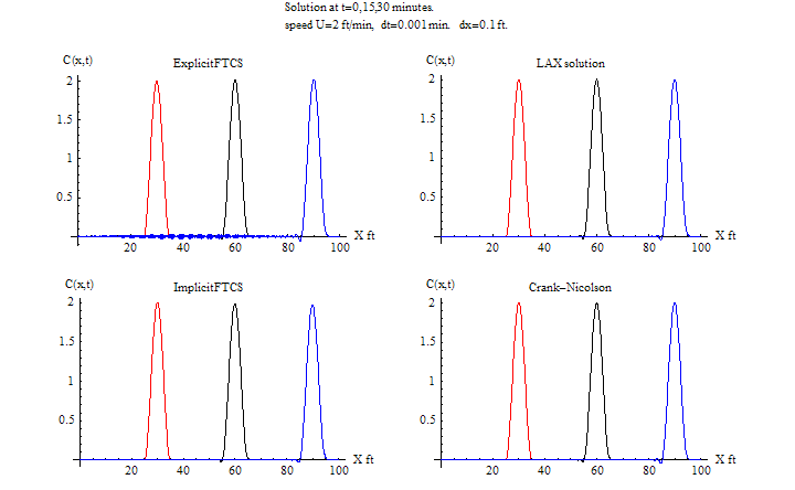
\(\tau =0.001\) sec, \(h=0.1\ ft\)
The explicit FTCS is stable for most of the run, near the end it is starting to be become unstable.
Notice that around 26 minutes that "bubbles" are starting to show up in the numerical solution downstream. This is a characteristic of how this method becomes unstable.
This will be more clear in the next test cases when the time step is made larger. For the varying speed case, the explicit method using the same time step remained stable during the whole 30 minutes. This is because the average speed was less than 2 ft/min, hence the mass did not have to travel as long a distance as with fixed speed of \(u=2\), and so the instability did not show up. Mathematically this can be explained by looking at the term \(\frac {u\tau }{h}\), hence for smaller \(u\), the courant number is smaller. Notice also the RMSE is smaller for variable speed compared to fixed speed. Again this is related to the smaller average speed making the courant number smaller.
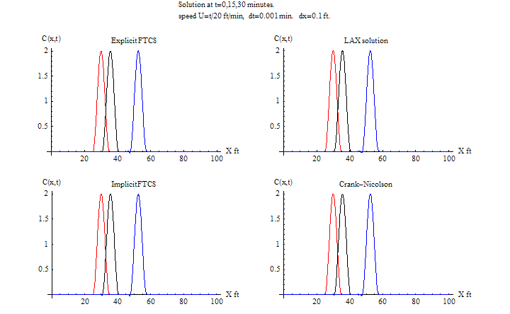
In this case, we slightly make the time step longer than before. We start to see the instability of FTCS.
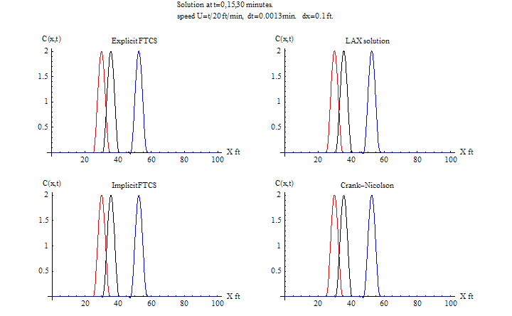
\(\tau =0.0013\) sec, \(h=0.1\ \)ft\(,\) \(\frac {u\tau }{h}=0.026\leq 1\) for fixed \(u\)
For explicit FTCS, The solution now starting to show instability at 25 minutes. Lax remained stable since CFL is satisfied. Explicit FTCS is becoming less accurate as well. Explicit Lax is most accurate at this time step.
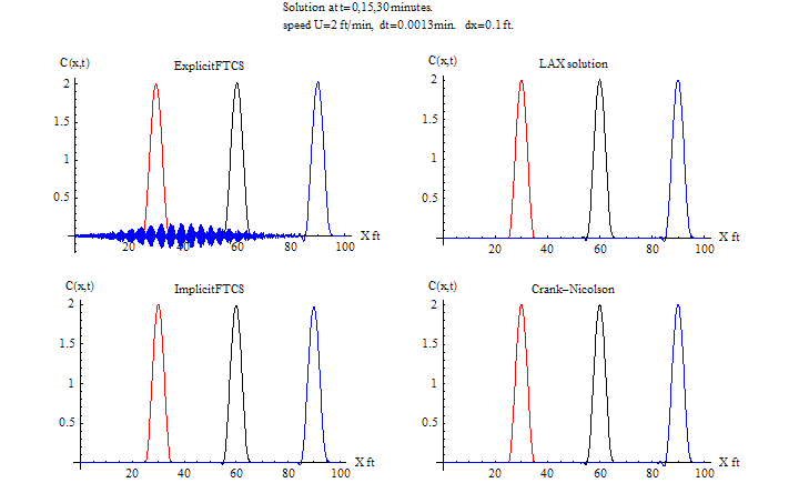
In this case, we slightly make the time step even longer than before. Now FTCS becomes more unstable.
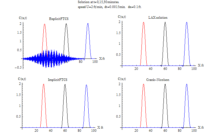
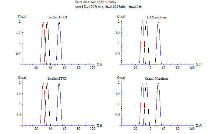
\(\tau =0.0015\) sec, \(h=0.1\ \)ft\(,\) \(\frac {u\tau }{h}=0.03\leq 1.\)
| Speed | Method | CPU time (sec) | RMSE | Animation (2D) | plots |
| U=2 | Explicit FTCS | 1.73 | 0.15249 | HTML | HTML |
| Explicit LAX | 2.56 | 0.000563 | HTML | ||
| Implicit FTCS | 3.34 | 0.009005 | HTML | ||
| C-R | 3.45 | 0.00565 | HTML | ||
| U=t/20 | Explicit FTCS | 1.84 | 0.00380 | HTML | HTML |
| Explicit LAX | 2.53 | 0.00336 | HTML | ||
| Implicit FTCS | 4,73 | 0.00358 | HTML | ||
| C-R | 5 | 0.003373 | HTML | ||
FTCS Instability starts at around 20 minutes. LAX remained stable since CFL is satisfied. Lax remained the most accurate at this time step. It accuracy actually improved as the time step became larger.
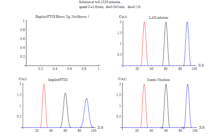
Again the time step is made longer than before. Now the explicit FTCS is completely unstable.
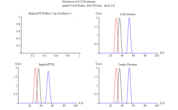
\(\tau =0.045\) sec, \(h=0.1\ \)ft
For the case of fixed \(U\), we have \(\frac {u\tau }{h}=\frac {2\times 0.045}{0.1}=\allowbreak 0.9\leq 1\), while for varying \(U\), the maximum value will be at the end of the run, which is \(30/20=1.5\) ft/min., hence the CFL condition is changing, with a value of \(\frac {1.5\times 0.045}{0.1}=\allowbreak 0.675\,\) at the end of the run which is still \(\leq 1\)
| Speed | Method | CPU time (sec) | RMSE | Animation (2D) | plots |
| U=2 | Explicit FTCS | 0.73 | blows up | HTML | HTML |
| Explicit LAX | 0.281 | 0.000162 | HTML | ||
| Implicit FTCS | 0.437 | 0.1306 | HTML | ||
| C-R | 0.4 | 0.01028 | HTML | ||
| U=t/20 | Explicit FTCS | 0.28 | blow up | HTML | HTML |
| Explicit LAX | 0.3 | 0.01117 | HTML | ||
| Implicit FTCS | 0.40 | 0.0386 | HTML | ||
| C-R | 0.4 | 0.01197 | HTML | ||
For the varying speed case, the explicit FTCS remained stable for the duration of the run as compared to the case with the fixed speed. This is because the average wave speed is less than with the fixed wave speed case.
The magnification factor depends on the speed of the wave.
\[ \left \vert \xi \right \vert =\sqrt {1+\left ( \frac {u\tau }{h}\sin \left ( kh\right ) \right ) ^{2}}\]
With the varying speed case, the coefficient \(\frac {u\tau }{h}\) was smaller during the whole run, since the maximum speed \(u\) attained will be \(1.5\,\ \)ft/min. as compared to \(2\) ft/min. in the fixed \(u\) case.
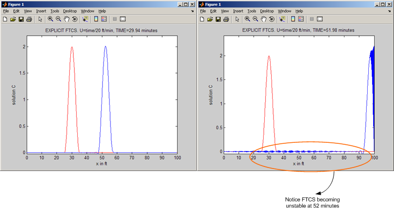
If we have run the simulation a little longer for the varying speed case, we will see the instability with explicit FTCS. This below is a diagram showing 2 runs using the explicit FTCS both with \(u=\frac {t}{20}\) ft/min, one was run for 30 minutes, and the second for 53 minutes. The run to 30 minutes showed no instability while the run for 53 minutes showed the instability. This show the explicit FTCS will eventually become unstable.
This is an animation of the above HTML
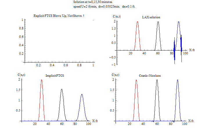
In this case, the time step is increased so that \(\frac {u\tau }{h}\) is just above the CFL condition.
Notice now that the Explicit LAX method become unstable as expected. The other implicit methods remain stable. the explicit FTCS method now is completely unstable. The implicit FTCS method is starting to become less accurate.
\(\tau =0.05025\) sec, \(h=0.1\ \)ft\(,\) \(\frac {u\tau }{h}=\frac {2\times 0.05025}{0.1}=1.005>1\)
| Speed | Method | CPU time (sec) | RMSE | Animation (2D) | plots |
| U=2 | Explicit FTCS | 0.7 | blows up | N/A blows up | HTML |
| Explicit LAX | 0.25 | 0.1006 | HTML | ||
| Implicit FTCS | 0.5 | 0.13945 | HTML | ||
| C-R | 0.468 | 0.01104 | HTML | ||
| U=t/20 | Explicit FTCS | 0.28 | blows up | N/A blows up | HTML |
| Explicit LAX | 0.31 | 0.04385 | HTML | ||
| Implicit FTCS | 0.45 | 0.0428 | HTML | ||
| C-R | 0.56 | 0.01317 | HTML | ||
Notice that explicit LAX takes much less CPU than any other method.
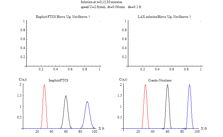
\(\tau =0.06\) sec, \(h=0.1\ \)ft\(,\) \(\frac {u\tau }{h}=\frac {2\times 0.06}{0.1}=1.2>1\)
| Speed | Method | CPU time (sec) | RMSE | Animation (2D) | plots |
| U=2 | Explicit FTCS | 0.65 | blows up | N/A blows up | HTML |
| Explicit LAX | 0.9 | blows up | HTML | ||
| Implicit FTCS | 0.42 | 0.1531 | HTML | ||
| C-R | 0.41 | 0.01244 | HTML | ||
| U=t/20 | Explicit FTCS | 0.265 | blows up | N/A blows up | HTML |
| Explicit LAX | 0.29 | 0.01389 | HTML | ||
| Implicit FTCS | 0.36 | 0.0493 | HTML | ||
| C-R | 0.36 | 0.01525 | HTML | ||
Notice that the CPU for the implicit method when speed is fixed is now higher than the CPU for the explicit methods. This can be explained as follows: since the time step now is larger than before, the number of times to solve \(Ax=b\) has been reduced. This made the implicit methods faster.
This implies that
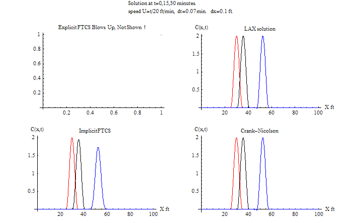
\(\tau =0.07\) sec, \(h=0.1\ \)ft\(,\) \(\frac {u\tau }{h}=\frac {2\times 0.07}{0.1}=1.4>1\)
| Speed | Method | CPU time (sec) | RMSE | Animation (2D) | plots |
| U=2 | Explicit FTCS | 0.5 | blows up | N/A blows up | HTML |
| Explicit LAX | 0.89 | blows up | HTML | ||
| Implicit FTCS | 0.453 | 0.1653 | HTML | ||
| C-R | 0.36 | 0.01403 | HTML | ||
| U=t/20 | Explicit FTCS | 0.234 | blows up | N/A blows up | HTML |
| Explicit LAX | 0.2187 | 0.01564 | HTML | ||
| Implicit FTCS | 0.344 | 0.0557 | HTML | ||
| C-R | 0.312 | 0.0174 | HTML | ||
As expected, CPU time usage will be less as the time step is increased. There is an anomaly cased noticed where the CPU time increased for the Lax method when the time step is increased from \(0.05025\) to \(0.06\,,\) This needs further investigation.
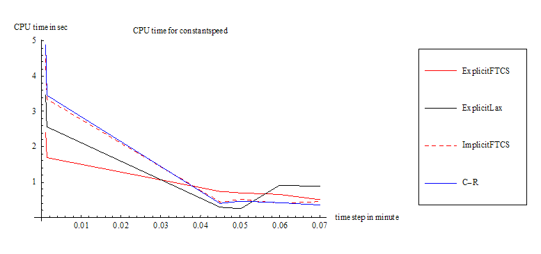
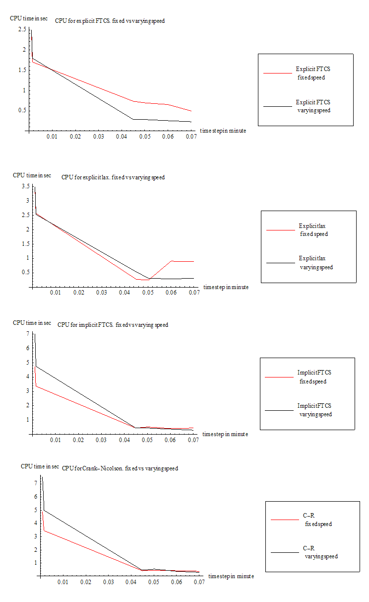
This table below summarizes the CPU time in seconds used by each method for the case of constant speed as time step is increased.
| \(\tau \ \ \ \sec \) | \(Explicit\ FTCS\) | \(Explicit\ LAX\) | \(Implicit\ FTCS\) | \(C-R\) |
| \(0.0001\) | \(20\) | \(31\) | \(45\) | \(49\) |
| \(0.001\) | \(2.42\) | \(3.48\) | \(4.7\) | \(4.9\) |
| \(0.0013\) | \(1.9\) | \(2.78\) | \(3.7\) | \(3.9\) |
| \(0.0015\) | \(1.7\) | \(2.56\) | \(3.34\) | \(3.45\) |
| \(0.045\) | \(0.73\) | \(0.281\) | \(0.43\) | \(0.4\) |
| \(0.05025\) | \(0.7\) | \(0.25\) | \(0.5\) | \(0.468\) |
| \(0.06\) | \(0.65\) | \(0.9\) | \(0.4\) | \(0.41\) |
| \(0.07\) | \(0.5\) | \(0.89\) | \(0.45\) | \(0.36\) |
This is the plot of the above table
This table below summarizes the CPU time in seconds used by each method for the case of varying speed as time step is increased.
| \(\tau \ \ \ \sec \) | \(Explicit\ FTCS\) | \(Explicit\ LAX\) | \(Implicit\ FTCS\) | \(C-R\) |
| \(0.0001\) | \(21\) | \(31\) | \(67\) | \(69\) |
| \(0.001\) | \(2.5\) | \(3.5\) | \(7\) | \(7.5\) |
| \(0.0013\) | \(2\) | \(2.9\) | \(5.56\) | \(6\) |
| \(0.0015\) | \(1.8\) | \(2.53\) | \(4.73\) | \(5\) |
| \(0.045\) | \(0.28\) | \(0.54\) | \(0.45\) | \(0.45\) |
| \(0.05025\) | \(0.28\) | \(0.31\) | \(0.45\) | \(0.56\) |
| \(0.06\) | \(0.265\) | \(0.29\) | \(0.36\) | \(0.36\) |
| \(0.07\) | \(0.23\) | \(0.22\) | \(0.33\) | \(0.31\) |
This is the plot of the above table
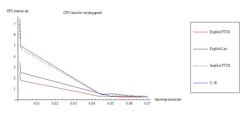
This plot below compares the CPU time for each method when the speed is constant vs. when the speed was changing with time.
This table below summarizes the RMS error from each numerical method as a function of changing the time step size. This is for case of constant speed.
| \(time\ step\) | \(Explicit\ FTCS\) | \(Explicit\ LAX\) | \(Implicit\ FTCS\) | \(C-R\) |
| \(0.0001\) | \(0.0546\) | \(0.0543\) | \(0.0548\) | \(0.0544\) |
| \(0.001\) | \(0.01264\) | \(0.0057\) | \(0.00742\) | \(0.00575\) |
| \(0.0013\) | \(0.0494\) | \(0.01125\) | \(0.01245\) | \(0.00128\) |
| \(0.0015\) | \(0.15249\) | \(0.00056\) | \(0.009\) | \(0.0056\) |
| \(0.045\) | \(blows\ up\) | \(0.000162\) | \(0.1306\) | \(0.01028\) |
| \(0.05025\) | \(blows\ up\) | \(0.1006\) | \(0.1394\) | \(0.011\) |
| \(0.06\) | \(blows\ up\) | \(blows\ up\) | \(0.1531\) | \(0.01244\) |
| \(0.07\) | \(blows\ up\) | \(blows\ up\) | \(0.1653\) | \(0.01403\) |
Notice that the Lax method became more accurate when the time step was increased from \(0.0001\) to \(0.04\) seconds, then it starts to become less accurate as time step is increased. This is counter intuitive to what one can expect. It will be interesting to investigate this further to obtain a mathematical explanation for this strange phenomena.
The accuracy of the implicit FTCS, and C-R also increased slightly as the time step became larger from \(0.0001\) to \(0.0015\), then the implicit FTCS became worst in terms of accuracy as the time step increased.
C-R method accuracy did not deteriorate as much with increasing the time step. This shows the C-R scheme to be more robust.
This table below summarizes the RMS error from each numerical method as a function of changing the time step size. This is for case of changing speed.
| \(time\ step\) | \(Explicit\ FTCS\) | \(Explicit\ LAX\) | \(Implicit\ FTCS\) | \(C-R\) |
| \(0.0001\) | \(0.003\) | \(0.003\) | \(0.003\) | \(0.0030\) |
| \(0.001\) | \(0.00352\) | \(0.00329\) | \(0.0033\) | \(0.0033\) |
| \(0.0013\) | \(0.00365\) | \(0.00331\) | \(0.00346\) | \(0.0033\) |
| \(0.0015\) | \(0.0038\) | \(0.00336\) | \(0.0035\) | \(0.00337\) |
| \(0.045\) | \(blows\ up\) | \(0.01117\) | \(0.0386\) | \(0.0119\) |
| \(0.05025\) | \(blows\ up\) | \(0.04385\) | \(0.0428\) | \(0.01317\) |
| \(0.06\) | \(blows\ up\) | \(0.01389\) | \(0.0493\) | \(0.01525\) |
| \(0.07\) | \(blows\ up\) | \(0.01564\) | \(0.0557\) | \(0.0174\) |
The effect of having the speed defined as \(\mu =\frac {t}{20}\)is to delay instability for the explicit methods as time step is increased. Notice also here the case where the Lax method became more accurate as the time step is increased from \(0.0001\) to \(0.0015\).
4 different numerical finite difference schemes are examined for CPU time, stability and accuracy in solving the advection PDE for constant speed and for a speed which is a function of time.
For accuracy, an interesting result is observed. The Lax scheme is the most accurate for Courant number close to unity. This means as the time step is increased, the Lax become more accurate of the 4 methods. But beyond the CFL condition, Both explicit methods (FTCS and Lax) became less accurate. Explicit FTCS became unstable sooner than Lax, while the implicit methods remained stable.
The implicit FTCS was less accurate than the C-R method. This implies that one should use the Lax method if one can be satisfied with a time step such that the courant number is close to a unit.
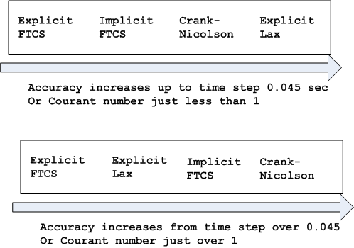
For stability, Crank-Nicolson was the most stable of all methods. Stability by itself is not sufficient condition to use to select a numerical scheme. It must also be accurate. The C-R method has both these properties for the range of the time steps considered. But as mentioned above, there is a range of time steps in which the Lax method is more accurate than all the other methods.
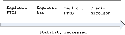
For CPU usage, the explicit methods used less CPU time when the time step was small, up to \(0.0015\sec .\) This can be explained as follows: for small step size, the number of time to solve \(Ax=b\,\) is large. Hence the implicit methods will be slower. As the time step is increased to the range of \(0.045\sec \) and over, the implicit methods actually became more CPU efficient due to the fact that the number of times to solve \(Ax=b\) is less because the number of steps is less.
In conclusion, the selection of a finite difference scheme depends on many factors. Stability and accuracy being the most important. The time step size plays a critical rule. For Courant number close to a unity, the Lax method is the most attractive. For larger time steps, the C-R method should be considered.


!*******************************************
!*
!* Solve the advection PDE using Explicit FTCS,
!* Explicit Lax, Implicit FTCS, and implicit Crank-Nicolson
!* methods for constant and varying speed.
!*
!*  Solve  dc/dt = -u dc/dx
!*  u = t/20 ft/minute
!*  and
!*  u constant
!*
!* Compiler used: gnu 95 (g95) on Cygwin. Gcc 3.4.4
!* Date: June 20 2006
!*
!* by Nasser Abbasi
!*******************************************

PROGRAM advection
  IMPLICIT NONE

  REAL     :: DT,DX,max_run_time,length,snapshot_delta, &
              first_limit,second_limit
  INTEGER  :: N,SNAPSHOTS
  character(10) :: cmd_arg ! to read time step from command line

  INTEGER :: method  ! 1=FTCS, 2=LAX, 3=Implicit FTCS, 4=C-R
  INTEGER :: mode    ! 1=Fixed wind speed, 2=speed function of time

  REAL    :: t_start, t_end, cpu_time_used,end_line(1002)
  INTEGER :: ALL_DATA_FILE_ID
  PARAMETER(ALL_DATA_FILE_ID=900)

  ! Initialize data. All methods will use the same
  ! parameters to make comparing them easier

  ! read delta t from command line.
  CALL getarg(1,cmd_arg)
  cmd_arg=TRIM(cmd_arg)
  print *,'= ', cmd_arg
  read(cmd_arg,*)dt   !delta in time,  in minutes

  print *,'Dt=',DT

  N      = 1000      ! number of grid points in space
  length = 100       ! length of space solution in feet

  first_limit  = 0.25*length
  second_limit = 0.35*length

  DX = length/N     ! delta in space, in feets

  max_run_time = 30.0  ! how long to run for in minutes
  SNAPSHOTS    = 200   ! number of snapshots per run. Used for animation

  snapshot_delta = max_run_time / SNAPSHOTS   ! time between each snap shot

  print *,'DT=',DT,' minutes, DX=',DX,' feets'
  print *,'taking snapshots every ', snapshot_delta ,' minutes'

  DO mode=1,2
     print*,'=======> processing mode ',mode
     DO method=1,4   ! No enumeration data types in Fotran 90

        CALL CPU_TIME(t_start)  ! get current CPU time
        CALL process(mode,method,N,DT,DX,max_run_time,snapshot_delta,&
             first_limit,second_limit)
        CALL CPU_TIME(t_end)    ! get current CPU time

        cpu_time_used = t_end - t_start

        WRITE(*,FMT='(A,I2,A,F12.5)') 'CPU TIME used for method', method, ' = ', cpu_time_used
        ! Now record test case parameters in last line
        end_line=0
        end_line(1)=cpu_time_used
        end_line(2)=DT
        end_line(3)=DX
        end_line(4)=mode
        end_line(5)=method

        WRITE(UNIT=ALL_DATA_FILE_ID,FMT=*) end_line
        CLOSE(ALL_DATA_FILE_ID)

     END DO
  END DO

END PROGRAM advection
!************************************
!*
!*
!************************************
SUBROUTINE process(mode,method,N,DT,DX,max_run_time,snapshot_delta,&
                   first_limit,second_limit)
  IMPLICIT NONE

  INTEGER, INTENT(IN) :: mode,method,N
  REAL,    INTENT(IN) :: DT,DX,max_run_time,snapshot_delta,&
                         first_limit,second_limit

  INTEGER :: I
  LOGICAL :: snap_shot_at_15_taken
  INTEGER :: ALL_DATA_FILE_ID
  PARAMETER(ALL_DATA_FILE_ID=900)
  REAL    :: snap_current_time
  REAL    :: current_time
  REAL    :: C(N)       ! current solution
  REAL    :: CNEW(N)    ! future solution
  REAL    :: CEXACT(N)  ! current exact solution
  REAL    :: current_first_limit
  REAL    :: A(N,N),aa(N),b(2:N),cc(N-1),CTEMP(N)  ! for C-R and implicit FTCS
  REAL    :: K,speed
  REAL    :: error,RMS   ! root mean square error between current and initial sol.

  current_time      = 0.
  snap_current_time = 0.

  CALL initialize_solution(C,N,DX,first_limit,second_limit)
  CEXACT = C
  current_first_limit = first_limit

  CALL pre_loop_initialization(mode,method,current_time,K, &
                               DT,DX,N,C,ALL_DATA_FILE_ID, &
                               A,aa,b,cc )

  snap_shot_at_15_taken=.FALSE.

  DO WHILE(current_time < max_run_time)

     IF( snap_current_time >= snapshot_delta ) THEN
        snap_current_time = 0.
        WRITE( UNIT=ALL_DATA_FILE_ID, FMT=*) current_time, error, C
     END IF

     SELECT CASE(method)

     CASE( 1:2 )

        IF(method==1) THEN  ! ftcs
           IF(mode==2)THEN
              K  = speed(mode,current_time)*DT/(2.*DX)
           ENDIF

           DO I = 2,N-1
              CNEW(I) = C(I) - K * ( C(I+1) - C(I-1) )
           END DO
        ELSE    !lax
           IF(mode == 2) THEN
              K = speed(mode,current_time)*DT/(DX)
           ENDIF

           DO I = 2,N-1
              CNEW(I) = C(I) - K/2. * ( C(I+1) - C(I-1) ) + &
                   (K**2.)/2 * ( C(I+1) +C(I-1)-2.*C(I) )
           END DO
        END IF

        CNEW(1) = C(1)
        CNEW(N) = C(N)  ! Boundary conditions
        C=CNEW

     CASE( 3 )  ! implicit ftcs

        IF( mode == 2) THEN ! only need to update Matrix for varying U
           K  = speed(mode,current_time)*DT/(2.*DX)

           CALL init_A_matrix(A,K,N)
           CALL init_diagonal_vectors(N,A,cc,aa,b)
        END IF

        CALL solve_thomas_algorithm(N,aa,b,cc,C,CNEW)
        C = CNEW

     CASE( 4 )   ! C-R

        IF(mode == 2) THEN  !only need to update A if U changes
           K  = speed(mode,current_time)*DT/(4*DX)   ! C-R
           CALL init_A_matrix(A,K,N)
           CALL init_diagonal_vectors(N,A,cc,aa,b)
        END IF

        CTEMP(1) = C(1)
        CTEMP(N) = C(N)

        DO I=2,N-1
           CTEMP(I)=C(I)+K*C(I-1)-K*C(I+1)
        END DO

        CALL solve_thomas_algorithm(N,aa,b,cc,CTEMP,C)

     END SELECT

     IF( current_time>=15.0 .AND. (.NOT. snap_shot_at_15_taken)) THEN
        snap_shot_at_15_taken = .TRUE.
        CALL take_one_snap_shot(mode,method,15,N,C,DX)
     END IF

     current_time = current_time + DT
     current_first_limit = current_first_limit + speed(mode,current_time)*DT
     CALL get_current_exact_solution(CEXACT,N,current_first_limit,DX)
     error = RMS(CEXACT,C,N)

     snap_current_time = snap_current_time + DT

  END DO

  CALL take_one_snap_shot(mode,method,30,N,C,DX)

END SUBROUTINE process
!************************************
!*
!*
!************************************
SUBROUTINE pre_loop_initialization(mode,method,current_time,K,&
                                   DT,DX,N,C,ALL_DATA_FILE_ID,&
                                   A,aa,b,cc)
  IMPLICIT NONE

  INTEGER, INTENT(IN)  :: mode,method,N,ALL_DATA_FILE_ID
  REAL,    INTENT(IN)  :: C(N),DT,DX,current_time
  REAL,    INTENT(OUT) :: K,A(N,N),aa(N),b(2:N),cc(N-1)
  REAL                 :: speed

  SELECT CASE(method)
  CASE( 1 )   ! FTCS

     K  = speed(mode,current_time)*DT/(2.*DX)

     IF(mode==1) THEN
        OPEN(UNIT=ALL_DATA_FILE_ID, file='expAll.txt') ! all time shots
        CALL print_to_file(C,'exp0.txt',N,DX)
     ELSE
        OPEN(UNIT=ALL_DATA_FILE_ID, file='exp_extraAll.txt') ! all time shots
        CALL print_to_file(C,'exp_extra0.txt',N,DX)
     END IF

  CASE( 2 )    ! Lax

     K = speed(mode,current_time)*DT/(DX)

     IF(mode==1) THEN
        OPEN(UNIT=ALL_DATA_FILE_ID, file='laxAll.txt') ! all time shots
        CALL print_to_file(C,'lax0.txt',N,DX)
     ELSE
        OPEN(UNIT=ALL_DATA_FILE_ID, file='lax_extraAll.txt') ! all time shots
        CALL print_to_file(C,'lax_extra0.txt',N,DX)
     END IF

  CASE( 3 )    ! Implicit FTCS

     K  = speed(mode,current_time)*DT/(2.*DX)

     CALL init_A_matrix(A,K,N)
     CALL init_diagonal_vectors(N,A,cc,aa,b)

     IF(mode==1) THEN
        OPEN(UNIT=ALL_DATA_FILE_ID, file='impAll.txt') ! all time shots
        CALL print_to_file(C,'imp0.txt',N,DX)
     ELSE
        OPEN(UNIT=ALL_DATA_FILE_ID, file='imp_extraAll.txt') ! all time shots
        CALL print_to_file(C,'imp_extra0.txt',N,DX)
     END IF

  CASE( 4 )     ! C-R

     K  = speed(mode,current_time)*DT/(4*DX)   ! C-R

     CALL init_A_matrix(A,K,N)
     CALL init_diagonal_vectors(N,A,cc,aa,b)

     IF(mode==1) THEN
        OPEN(UNIT=ALL_DATA_FILE_ID, file='crAll.txt') ! all time shots
        CALL print_to_file(C,'cr0.txt',N,DX)
     ELSE
        OPEN(UNIT=ALL_DATA_FILE_ID, file='cr_extraAll.txt') ! all time shots
        CALL print_to_file(C,'cr_extra0.txt',N,DX)
     END IF
  END SELECT

  WRITE( UNIT=ALL_DATA_FILE_ID, FMT=*) current_time,0, C

END SUBROUTINE pre_loop_initialization
!************************************
!*
!*
!************************************
SUBROUTINE init_diagonal_vectors(N,A,cc,aa,b)
  IMPLICIT NONE

  INTEGER, INTENT(IN) ::N
  REAL, INTENT(IN)    ::A(N,N)
  REAL, INTENT(OUT)   ::aa(N),b(2:N),cc(N-1)

  INTEGER ::I,J

  J=2
  DO I=1,N-1
     cc(I)=A(I,J)
     J=J+1
  END DO
  cc(1)=0

  DO I=1,N
     aa(I)=A(I,I)
  END DO

  J=1
  DO I=2,N
     b(I)=A(I,J)
     J=J+1
  END DO

END SUBROUTINE init_diagonal_vectors
!************************************
!*
!*
!************************************
SUBROUTINE initialize_solution(C,N,DX,first_limit,second_limit)
  IMPLICIT NONE

  INTEGER, INTENT(IN)    :: N
  REAL,    INTENT(IN)    :: DX,first_limit,second_limit
  REAL,    INTENT(INOUT) :: C(0:N-1)

  INTEGER :: I
  REAL    :: x, PI,av,R

  PARAMETER( PI = ACOS(-1.) )

  x = 0
  av = (second_limit+first_limit)/2.0
  R  = av - first_limit

  C = 0.0

  DO I=0,N-1

     IF( x >= first_limit .AND. x <= second_limit ) THEN
        C(I) = 1 + COS( PI * (x-av)/R )
     END IF

     x = x + DX
  END DO

END SUBROUTINE initialize_solution
!************************************
!*
!*
!************************************
SUBROUTINE print_to_file(C,file_name,N,DX)
  IMPLICIT NONE


  REAL,    INTENT(IN) :: C(N),DX
  INTEGER, INTENT(IN) :: N

  CHARACTER* (*), INTENT(IN) :: file_name

  INTEGER :: I
  INTEGER :: FILE_ID
  PARAMETER(FILE_ID=999)
  REAL :: current_position

  OPEN(UNIT=FILE_ID, file=file_name)

  current_position = 0;
  DO I=1,N

     WRITE( UNIT=FILE_ID, FMT=* ) current_position ,'' t', C(I)
     current_position = current_position + DX

  END DO

  CLOSE(FILE_ID)

END SUBROUTINE print_to_file
!************************************
!*
!*
!************************************
SUBROUTINE init_A_matrix(A,K,N)
  IMPLICIT NONE

  INTEGER, INTENT(IN) ::N
  REAL, INTENT(IN)    ::K
  REAL, INTENT(OUT)   ::A(N,N)

  INTEGER ::I

  DO I = 2,N-1
     A(I,I-1)   = -K
     A(I,I) = 1
     A(I,I+1) = K
  END DO

  A(1,1) = 1
  A(N,N) = 1

END SUBROUTINE init_A_matrix
!************************************
!*
!*
!************************************
SUBROUTINE solve_thomas_algorithm(N,aa,b,c,old_c,new_c)
  IMPLICIT NONE

  REAL, INTENT(IN)    :: aa(N),b(2:N),c(N-1),old_c(N)
  INTEGER, INTENT(IN) :: N
  REAL, INTENT(INOUT) :: new_c(N)

  INTEGER  :: I
  REAL :: alpha(N),beta(2:N),g(N)

  alpha(1) = aa(1)
  DO I=2,N
     beta(I)=b(I)/alpha(I-1)
     alpha(I)=aa(I)-beta(I)*c(I-1)
  END DO

  g(1)=old_c(1)
  DO I=2,N
     g(I)=old_c(I)-beta(I)*g(I-1)
  END DO

  new_c(N)=g(N)/alpha(N)
  DO I=N-1,1,-1
     new_c(I)=(g(I)-c(I)*new_c(I+1))/alpha(I)
  END DO

END SUBROUTINE solve_thomas_algorithm
!************************************
!*
!*
!************************************
REAL FUNCTION speed(MODE,time)
  IMPLICIT NONE

  INTEGER, INTENT(IN) :: MODE
  REAL,    INTENT(IN) :: time

  IF( MODE == 1 ) THEN
     speed=2.0
  ELSE
     speed=time/20.0
  END IF

END FUNCTION speed
!************************************
!*
!*
!************************************
SUBROUTINE take_one_snap_shot(mode,method,TIME,N,C,DX)
  IMPLICIT NONE

  INTEGER, INTENT(IN) ::TIME,mode,method,N
  REAL,    INTENT(IN) ::C(N),DX

  IF(TIME==15) THEN
     SELECT CASE(method)
     CASE(1)
        IF(mode==1) THEN
           CALL print_to_file(C,'exp15.txt',N,DX)
        ELSE
           CALL print_to_file(C,'exp_extra15.txt',N,DX)
        END IF
     CASE(2)
        IF(mode==1) THEN
           CALL print_to_file(C,'lax15.txt',N,DX)
        ELSE
           CALL print_to_file(C,'lax_extra15.txt',N,DX)
        ENDIF
     CASE(3)
        IF(mode==1) THEN
           CALL print_to_file(C,'imp15.txt',N,DX)
        ELSE
           CALL print_to_file(C,'imp_extra15.txt',N,DX)
        END IF
     CASE(4)
        IF(mode==1) THEN
           CALL print_to_file(C,'cr15.txt',N,DX)
        ELSE
           CALL print_to_file(C,'cr_extra15.txt',N,DX)
        END IF
     END SELECT
  ELSE
     SELECT CASE(method)
     CASE(1)
        IF(mode==1) THEN
           CALL print_to_file(C,'exp30.txt',N,DX)
        ELSE
           CALL print_to_file(C,'exp_extra30.txt',N,DX)
        END IF
     CASE(2)
        IF(mode==1) THEN
           CALL print_to_file(C,'lax30.txt',N,DX)
        ELSE
           CALL print_to_file(C,'lax_extra30.txt',N,DX)
        ENDIF
     CASE(3)
        IF(mode==1) THEN
           CALL print_to_file(C,'imp30.txt',N,DX)
        ELSE
           CALL print_to_file(C,'imp_extra30.txt',N,DX)
        END IF
     CASE(4)
        IF(mode==1) THEN
           CALL print_to_file(C,'cr30.txt',N,DX)
        ELSE
           CALL print_to_file(C,'cr_extra30.txt',N,DX)
        END IF
     END SELECT
  END IF
END SUBROUTINE    take_one_snap_shot
!************************************
!*
!*
!************************************
REAL FUNCTION RMS(CEXACT,C,N)
  IMPLICIT NONE

  REAL, INTENT(IN)    :: CEXACT(N),C(N)
  INTEGER, INTENT(IN) :: N

  INTEGER  :: I

  RMS=0.
  DO I=1,N
     RMS = RMS+(CEXACT(I)-C(I))**2
  END DO

  RMS = RMS/N
  RMS = SQRT(RMS)
END FUNCTION RMS
!************************************
!*
!*
!************************************
SUBROUTINE get_current_exact_solution(CEXACT,N,current_first_limit,DX)
  IMPLICIT NONE
  REAL, INTENT(IN)    :: current_first_limit,DX
  REAL, INTENT(OUT)   :: CEXACT(0:N-1)
  INTEGER, INTENT(IN) :: N

  INTEGER :: I
  REAL :: first_limit
  REAL :: second_limit
  REAL :: av,R,shift,x,PI

  PARAMETER( PI = ACOS(-1.) )

  first_limit  = 25.0
  second_limit = 35.0

  shift = current_first_limit - FIRST_LIMIT
  first_limit = current_first_limit
  second_limit = second_limit + shift

  av = (second_limit+first_limit)/2.0
  R  = av - first_limit

  CEXACT = 0.
  x = 0.
  DO I = 0,N-1

     IF( x >= first_limit .AND. x <= second_limit ) THEN
        CEXACT(I) = 1 + COS( PI * (x -av)/R )
     END IF

     x = x + DX
  END DO
END SUBROUTINE get_current_exact_solution
1Richtmyer and Morton 1967. p45): "Given a properly posed linear initial value problem and a finite difference approximation to it that satisfies the consistency condition, stability is the necessary and sufficient condition for convergence."