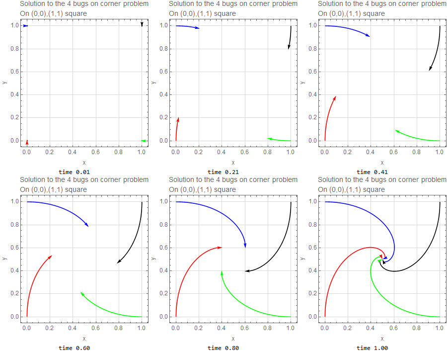
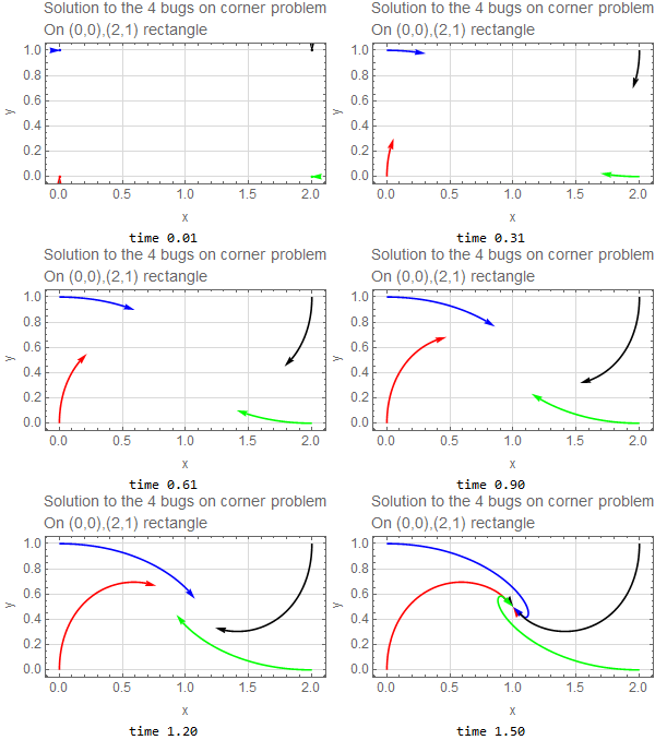
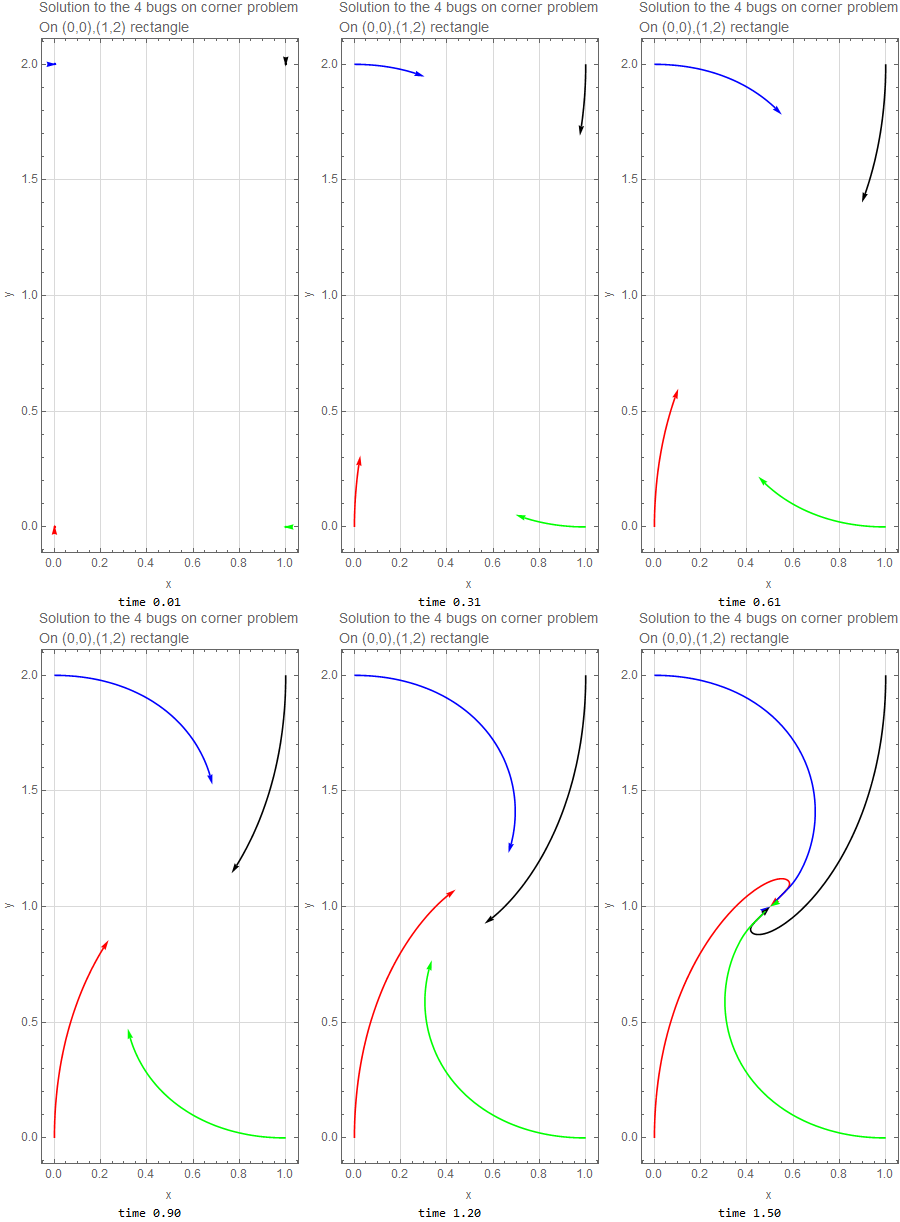
Four bugs on corners of a rectangle are standing at positions \(\left ( 0,0\right ) ,\left ( 0,2\right ) ,\left ( 1,2\right ) ,\left ( 1,0\right ) \). Bug 1 starts to move directly towards bug 2, while bug 2 moves directly towards bug 3 and bug 3 moves directly towards bug 4 and bug 4 moves directly towards bug 1. All are moving with unit speed. Motion is clockwise. Find the equations of motions and make animation of the motion.
The following diagram shows the initial positions of all four bugs and what happens after \(\Delta t\) has elapsed.
The four bugs are initially located at corners of rectangle. The width is \(h=1\) and the height is \(L=2\). Since each bug moves with the same speed toward the bug next to it (clockwise), then by symmetry, the four bugs will remain on the corners of a rectangle as time passes, but the rectangle will become smaller and rotate clockwise as the bugs spiral towards the center of the original rectangle where they all meet. The following diagram illustrates such motion after some \(\Delta t\) has elapsed.
We see that at each instance of time, each bug remains at the corner of a scaled down version of the original rectangle, which is rotating and the bug’s velocity is straight toward the bug position it is chasing. What this means is that bug 1 motion is always at \(90^{0}\) to the path of bug 2. And bug 2 motion is at \(90^{0}\) to the path of bug 3 and so on.
To obtain the equation of motion for each bug, we will look at each bug’s position relative to the bug it is chasing. Starting with bug 1 relative to bug 2 with the help of the following diagram
The position vector of bug 1 is \(\vec {r}_{1}\left ( t\right ) \) and the position vector of bug 2 is \(\vec {r}_{2}\left ( t\right ) \). Therefore \(\vec {v}_{1}=\frac {d\vec {r}_{1}\left ( t\right ) }{dt}=\left \vert \vec {v}_{1}\right \vert \hat {r}\) where \(\hat {r}\) is unit vector in the direction from bug 1 to bug 2. Hence\[ \frac {d\vec {r}_{1}\left ( t\right ) }{dt}=\left \vert \vec {v}_{1}\right \vert \frac {\vec {r}_{2}\left ( t\right ) -\vec {r}_{1}\left ( t\right ) }{\parallel \vec {r}_{2}\left ( t\right ) -\vec {r}_{1}\left ( t\right ) \parallel }\] But since \(\left \vert \vec {v}_{1}\right \vert =1\) meter per seconds then\begin {align*} \frac {d\vec {r}_{1}\left ( t\right ) }{dt} & =\frac {\left ( x_{2}\hat {\imath }+y_{2}\hat {\jmath }\right ) -\left ( x_{1}\hat {\imath }+y_{1}\hat {\jmath }\right ) }{\parallel \left ( x_{2}\hat {\imath }+y_{2}\hat {\jmath }\right ) -\left ( x_{1}\hat {\imath }+y_{1}\hat {\jmath }\right ) \parallel }\\ \left ( \frac {dx_{1}}{dt}\hat {\imath }+\frac {dy_{1}}{dt}\hat {\jmath }\right ) & =\frac {x_{2}-x_{1}}{\sqrt {\left ( x_{2}-x_{1}\right ) ^{2}+\left ( y_{2}-y_{1}\right ) ^{2}}}\hat {\imath }+\frac {y_{2}-y_{1}}{\sqrt {\left ( x_{2}-x_{1}\right ) ^{2}+\left ( y_{2}-y_{1}\right ) ^{2}}}\hat {\jmath } \end {align*}
Where \(x_{1},y_{1}\) are the coordinates of bug 1 and \(x_{2},y_{2}\) are the coordinates of bug 2. From the above, we obtain equations of motion for bug 1, where now we use \(x_{1}^{\prime }=\frac {dx}{dt}\) and \(y_{1}^{\prime }=\frac {dy}{dt}\) for bug 1.\begin {align} x_{1}^{\prime } & =\frac {x_{2}-x_{1}}{\sqrt {\left ( x_{2}-x_{1}\right ) ^{2}+\left ( y_{2}-y_{1}\right ) ^{2}}}\nonumber \\ y_{1}^{\prime } & =\frac {y_{2}-y_{1}}{\sqrt {\left ( x_{2}-x_{1}\right ) ^{2}+\left ( y_{2}-y_{1}\right ) ^{2}}}\tag {3} \end {align}
The same analysis is now done to obtain \(x_{2}^{\prime }\left ( t\right ) \) and \(y_{2}^{\prime }\left ( t\right ) \) expressions similar to (3) above for bug 2.
The position vector of bug 2 is \(\vec {r}_{2}\left ( t\right ) \) and the position vector of bug 3 is \(\vec {r}_{3}\left ( t\right ) \). Therefore \(\vec {v}_{2}=\frac {d\vec {r}_{2}\left ( t\right ) }{dt}=\left \vert \vec {v}_{2}\right \vert \hat {r}\) where \(\hat {r}\) is unit vector in the direction from bug 2 to bug 3. Hence\[ \frac {d\vec {r}_{2}\left ( t\right ) }{dt}=\left \vert \vec {v}_{2}\right \vert \frac {\vec {r}_{3}\left ( t\right ) -\vec {r}_{2}\left ( t\right ) }{\parallel \vec {r}_{3}\left ( t\right ) -\vec {r}_{2}\left ( t\right ) \parallel }\] Since \(\left \vert \vec {v}_{2}\right \vert =1\) meter per seconds then\begin {align*} \frac {d\vec {r}_{2}\left ( t\right ) }{dt} & =\frac {\left ( x_{3}\hat {\imath }+y_{2}\hat {\jmath }\right ) -\left ( x_{3}\hat {\imath }+y_{2}\hat {\jmath }\right ) }{\parallel \left ( x_{3}\hat {\imath }+y_{2}\hat {\jmath }\right ) -\left ( x_{3}\hat {\imath }+y_{2}\hat {\jmath }\right ) \parallel }\\ \left ( \frac {dx_{2}}{dt}\hat {\imath }+\frac {dy_{2}}{dt}\hat {\jmath }\right ) & =\frac {x_{3}-x_{2}}{\sqrt {\left ( x_{3}-x_{2}\right ) ^{2}+\left ( y_{3}-y_{2}\right ) ^{2}}}\hat {\imath }+\frac {y_{3}-y_{2}}{\sqrt {\left ( x_{3}-x_{2}\right ) ^{2}+\left ( y_{3}-y_{2}\right ) ^{2}}}\hat {\jmath } \end {align*}
Where \(x_{2},y_{2}\) are the coordinates of bug 2 and \(x_{3},y_{3}\) are the coordinates of bug 3. The above gives the two equations of motion for bug 2, where now we use \(x_{2}^{\prime }=\frac {dx_{2}}{dt}\) and \(y_{2}^{\prime }=\frac {dy_{2}}{dt}\) for bug 2.\begin {align} x_{2}^{\prime } & =\frac {x_{3}-x_{2}}{\sqrt {\left ( x_{3}-x_{2}\right ) ^{2}+\left ( y_{3}-y_{2}\right ) ^{2}}}\nonumber \\ y_{2}^{\prime } & =\frac {y_{3}-y_{2}}{\sqrt {\left ( x_{3}-x_{2}\right ) ^{2}+\left ( y_{3}-y_{2}\right ) ^{2}}}\tag {3} \end {align}
By doing the above again for bug 3 and bug 4, it is clear the result will be similar. The final equations of motions in vector form are\begin {align*} \mathbf {x}^{\prime } & =f\left ( \mathbf {x}\right ) \\ & \begin {pmatrix} x_{1}^{\prime }\left ( t\right ) =\frac {x_{2}-x_{1}}{\sqrt {\left ( x_{2}-x_{1}\right ) ^{2}+\left ( y_{2}-y_{1}\right ) ^{2}}}\\ y_{1}^{\prime }\left ( t\right ) =\frac {y_{2}-y_{1}}{\sqrt {\left ( x_{2}-x_{1}\right ) ^{2}+\left ( y_{2}-y_{1}\right ) ^{2}}}\\ x_{2}^{\prime }\left ( t\right ) =\frac {x_{3}-x_{2}}{\sqrt {\left ( x_{3}-x_{2}\right ) ^{2}+\left ( y_{3}-y_{2}\right ) ^{2}}}\\ y_{2}^{\prime }\left ( t\right ) =\frac {y_{3}-y_{2}}{\sqrt {\left ( x_{3}-x_{2}\right ) ^{2}+\left ( y_{3}-y_{2}\right ) ^{2}}}\\ x_{3}^{\prime }\left ( t\right ) =\frac {x_{4}-x_{3}}{\sqrt {\left ( x_{4}-x_{3}\right ) ^{2}+\left ( y_{4}-y_{3}\right ) ^{2}}}\\ y_{3}^{\prime }\left ( t\right ) =\frac {y_{4}-y_{3}}{\sqrt {\left ( x_{4}-x_{3}\right ) ^{2}+\left ( y_{4}-y_{3}\right ) ^{2}}}\\ x_{4}^{\prime }\left ( t\right ) =\frac {x_{1}-x_{4}}{\sqrt {\left ( x_{1}-x_{4}\right ) ^{2}+\left ( y_{1}-y_{4}\right ) ^{2}}}\\ y_{4}^{\prime }\left ( t\right ) =\frac {y_{1}-y_{4}}{\sqrt {\left ( x_{1}-x_{4}\right ) ^{2}+\left ( y_{1}-y_{4}\right ) ^{2}}}\end {pmatrix} \end {align*}
With initial conditions\[ \mathbf {x}\left ( 0\right ) =\begin {pmatrix} x_{1}\left ( 0\right ) \\ y_{1}\left ( 0\right ) \\ x_{2}\left ( 0\right ) \\ y_{2}\left ( 0\right ) \\ x_{3}\left ( 0\right ) \\ y_{3}\left ( 0\right ) \\ x_{4}\left ( 0\right ) \\ y_{4}\left ( 0\right ) \end {pmatrix} =\begin {pmatrix} 0\\ 0\\ 0\\ 2\\ 1\\ 2\\ 1\\ 0 \end {pmatrix} \] We can not write this as \(\mathbf {x}^{\prime }=A\mathbf {x}\) since it is not linear system. These ODE’s have to solved numerically since they are nonlinear. The following is the result of running the solution for \(1.5\) seconds with the code listing below it. This shows the bug spiraling down to the center of the original rectangle as expected.
This problem was also solved for a square instead of a rectangle. The only change needed was to make the initial conditions as follows\[ \mathbf {x}\left ( 0\right ) =\begin {pmatrix} x_{1}\left ( 0\right ) \\ y_{1}\left ( 0\right ) \\ x_{2}\left ( 0\right ) \\ y_{2}\left ( 0\right ) \\ x_{3}\left ( 0\right ) \\ y_{3}\left ( 0\right ) \\ x_{4}\left ( 0\right ) \\ y_{4}\left ( 0\right ) \end {pmatrix} =\begin {pmatrix} 0\\ 0\\ 0\\ 1\\ 1\\ 1\\ 1\\ 0 \end {pmatrix} \] The time needed to reach the center in this case is one second.
These animations will play in HTML only

|

|

|
Code for animation is
ClearAll[t, x1, x2, x3, x4, y1, y2, y3, y4];
ode1 = x1'[t] == (x2[t] - x1[t])/
   Sqrt[(x2[t] - x1[t])^2 + (y2[t] - y1[t])^2];
ode2 = y1'[t] == (y2[t] - y1[t])/
   Sqrt[(x2[t] - x1[t])^2 + (y2[t] - y1[t])^2];
ode3 = x2'[t] == (x3[t] - x2[t])/
   Sqrt[(x3[t] - x2[t])^2 + (y3[t] - y2[t])^2];
ode4 = y2'[t] == (y3[t] - y2[t])/
   Sqrt[(x3[t] - x2[t])^2 + (y3[t] - y2[t])^2];
ode5 = x3'[t] == (x4[t] - x3[t])/
   Sqrt[(x4[t] - x3[t])^2 + (y4[t] - y3[t])^2];
ode6 = y3'[t] == (y4[t] - y3[t])/
   Sqrt[(x4[t] - x3[t])^2 + (y4[t] - y3[t])^2];
ode7 = x4'[t] == (x1[t] - x4[t])/
   Sqrt[(x1[t] - x4[t])^2 + (y1[t] - y4[t])^2];
ode8 = y4'[t] == (y1[t] - y4[t])/
   Sqrt[(x1[t] - x4[t])^2 + (y1[t] - y4[t])^2];

sol = NDSolve[{ode1, ode2, ode3, ode4, ode5, ode6, ode7, ode8,
    x1[0] == 0, y1[0] == 0, x2[0] == 0, y2[0] == 1, x3[0] == 1,
    y3[0] == 1, x4[0] == 1, y4[0] == 0}, {x1[t], y1[t], x2[t], y2[t],
    x3[t], y3[t], x4[t], y4[t]}, {t, 0, 1}];

Manipulate[
 p1 = ParametricPlot[{x1[t], y1[t]} /. sol, {t, 0, tMax},
    AxesOrigin -> {0, 0}, GridLines -> Automatic,
    GridLinesStyle -> LightGray, Frame -> True,
    FrameLabel -> {{"y", None}, {"x", None}}, ImageSize -> 350,
    PlotStyle -> Red] /. Line[x_] :> {Arrowheads[.04], Arrow[x]};

 p2 = ParametricPlot[{x2[t], y2[t]} /. sol, {t, 0, tMax},
    AxesOrigin -> {0, 0}, GridLines -> Automatic,
    GridLinesStyle -> LightGray, Frame -> True,
    FrameLabel -> {{"y", None}, {"x", None}}, ImageSize -> 350,
    PlotStyle -> Blue] /. Line[x_] :> {Arrowheads[.04], Arrow[x]};

 p3 = ParametricPlot[{x3[t], y3[t]} /. sol, {t, 0, tMax},
    AxesOrigin -> {0, 0}, GridLines -> Automatic,
    GridLinesStyle -> LightGray, Frame -> True,
    FrameLabel -> {{"y", None}, {"x", None}}, ImageSize -> 350,
    PlotStyle -> Black] /. Line[x_] :> {Arrowheads[.04], Arrow[x]};

 p4 = ParametricPlot[{x4[t], y4[t]} /. sol, {t, 0, tMax},
    AxesOrigin -> {0, 0}, GridLines -> Automatic,
    GridLinesStyle -> LightGray, Frame -> True,
    FrameLabel -> {{"y", None}, {"x", None}}, ImageSize -> 350,
    PlotStyle -> Green] /. Line[x_] :> {Arrowheads[.04], Arrow[x]};

 Show[p1, p2, p3, p4, PlotRange -> {{0, 1}, {0, 1}},
  PlotLabel ->
   Column[{"Solution to the 4 bugs on corner problem",
     "On (0,0),(1,1) square"}], BaseStyle -> 12, ImageSize -> 300],

 {{tMax, .01, "time"}, .01, 1, .01, Appearance -> "Labeled"}
 ]